Download
1 / 39
390 likes | 478 Vues
Learn about star-join schemas, fact tables, partitioning strategies, value chains, data warehouse problems, integration, and design process in data warehousing.

E N D
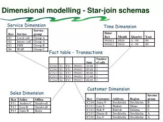
Dimensional modelling - Star-join schemas Service Dimension Time Dimension Fact table - Transactions Number Sum of calls C210 S1 F11 991011 25:00 3 C210 S3 F11 991011 05:00 1 C212 S2 F13 991011 89:00 1 C213 S1 F13 991011 12:00 1 C214 S4 F13 991012 08:00 1 Customer Dimension Sales Dimension
Partitioning strategy • for performace-related and manageablity reasons • usually for handling the fact table Horisontal partitioning - speed up queries by minimising the data to be scanned (without using an index) - partition by time most common Vertical partitioning - data is split vertically - two forms: normalisation and row splitting - consider row splitting if some columns are access infrequently Dim Fact Dim Dim
A family of stars • A dimensional model of a data warehouse for a large data warehouse consists of between 10 and 25 similar-looking star-join schemas. Each star join will have 5 to 15 dimensional tables. • Conformed (shared) dimensions for drill-across. A Conformed dimension is a dimension that means the same thing with every possible fact table to which it can be joined.
Value chains as families of star-join schemas • There are two sides to the value chain • the demand side- the steps needed to satisfy the customers’ demand for the product • the supply side - the steps needed to manufacture the products from original ingredients or parts • The chain consists of a sequence of inventory and flow star-join schemata • joining the different star-join schemata is only possible when two sequential schemata have a common, identical dimension • Sometimes the represented chain can be extended beyond the bounds of the business itself
Supply Chain Row material production Ingredient purchasing Ingredient delivery Ingredient inventory Bill of materials Manufacturing process control Manufacturing costs Packaging Trans-shipping to warehouse Finished goods inventory Demand Chain Finished goods inventory Manufacturing shipments Distributor inventory Distributor shipments Retail inventory Retail sales Value chains as families of star-join schemas
The Data Warehouse Bus Orders Production Dimensions Time Sales Rep Customer Promotion Product Plant Distr. Center
Problems of Data Warehousing • Complexity of integration • Hidden problems with source systems • Data homogenisation • Underestimation of resources for data loading • Required data not captured • High maintenance • Long duration projects • Why not integrating the legacy applications (OLTP systems) instead?
The stove pipe problem IT system5 IT- system4 IT- system3 IT- system2 IT- system1 Market Purchase Production Shipment Service Business process
The stove pipe problem IT system5 IT- system4 IT- system3 IT- system2 IT- system1 IT systems Market Purchase Production Shipment Service Business process
Integrating the Enterprise - ERP/ES & DW Managers Customers Suppliers Reporting and DW Sales force Finan- cials Sales & delivery Back office Manufac- turing Central database Services Inventory Human resource Customer service Employees
case Integration of Telecom systems - point-to-point
Integration of Telecom systems - Message Brokers & DW DW Message Broker
Dimensional modelling vs. ER-modelling Entity-relationship modelling - a logical design technique to eliminate data redundancy to keep consistency and storage efficiency - makes transaction simple and deterministic - ER models for enterprise are usually complex, e.g. they often have hundreds, or even thousands, of entities/tables Dimensional modelling - a logical design technique that present data in a intuitive way and that allow high-performance access - aims at model decision support data - easier to navigate for the user and high performance
Why dimensional modelling? • the logical model is easy understand • a predictable standard framework for end user applications • the logical design can be done nearly independent of expected query pattern • handle changes easy - at least adding new dimensional attributes • high performance “browsing” across the attributes, eliminating joins and make use bit vector indexes • strategy to handling aggregates, e.g. summery records that are logical redundant with base table to enhance query performance • the database engine can make strong assumption how to optimise • strategies for handling slowly changing dimensions, heterogenous products, event-handling (“factless fact tables”)
Steps in the Design Process 1 Choose a business process to model A business process is a major operational process in an organi-sation, that is supported by some kind of a legacy system(s) from which data can be collected, e.g., orders, invoices, shipments, inventory. 2 Choose the grain of the business process The grains is the level of detail at which the data is represented in the DW. Typical grains areindividual transactions, individual daily (monthly) snapshots. 3 Choose the dimensions that will apply to each fact table record Typical dimensions aretime, product, customer, store, etc. 4 Choose the measured facts that will populate fact table E.g., quantity sold, dollars sold
Consider the following questions • How much total business did my newly remodelled stores do compared with the chain average? • How did leather goods items costing less than $5 do with my most frequent shoppers? • What was the ratio of nonholiday weekend days total revenue to holiday weekend days?
Aggregation • Aggregations can be created on-the-fly or by the process of pre-aggregation • An aggregate is a fact table record representing a summarisation of base-level fact table records • Category-levelproduct aggregates by store by day • District-levelstore aggregates by product by day • Monthly sales aggregates by product by store • Category-level product aggregates by store district by day • Category-level product aggregates by store district by month
How to store aggregates • as new Level fields in an already existing Fact table • as new fact tables
New Level field for Aggregates NB! Constraint the queries to avoid double counting of the Level fields
An example ? $sold napkin/day ? $sold tissue/day ? $sold paper/day
New Level field for Aggregates - an example ? $sold napkin/day ? $sold tissue/day ? $sold paper/day Well, is this a solution you would chose?
New Fact Tables for Aggregates The creation of aggregate fact table requires the creation of: a derivative dimension an artificial key for each new derivative dimension
How to store aggregates • as new Level fields in an already existing Fact table • problems with double count • visible for the users • as new fact tables + no problems with double count + invisible for the users + are easily introduced and/or reduced at different points in time + simpler metadata + simpler choice of key + the size of the field for the summarised data does not increase the size of the field for the basic data
Sparsity Failure The planning of aggregate table sizes can be tricky because of the phenomenon called sparsity failure This phenomenon appears when we build aggregates on sparse tables. For example: In the grocery store item movement database, only about 10% of the products in the store are actually sold in a given store on a given day. Even disregarding the promotion dimension, the database is only occupied 10% in the primary keys of product, store, and time. However when we build aggregates, the occupancy rate shoots up dramatically.
Aggregation Navigator Query Tool Client or Application Server base level SQL aggregated results Aggregation Metadata Aggregate Navigator aggregate-aware SQL aggregated results DBMS data + aggregations
An example of SQL query category_sales_fact category_product SELECT category_description, sum(sales_dollars) FROM base_sales_fact, product, store, time WHERE base_sales_fact.product_key = product.product_key AND base_sales_fact.store_key = store.store_key AND base_sales_fact.time_key = time.time_key AND store.city = ‘Cincinnati’ AND time.day = ‘January 1, 1996’ GROUPBY category_description
An example of SQL query, cont SELECT category_description, sum(sales_dollars) FROMcategory_sales_fact, category_product, store, time WHEREcategory_sales_fact.product_key = category_product.product_key ANDcategory_sales_fact.store_key = store.store_key ANDcategory_sales_fact.time_key = time.time_key AND store.city = ‘Cincinnati’ AND time.day = ‘January 1, 1996’ GROUPBY category_description
Aggregation Navigator • Insulates end user applications from the changing portfolio of aggregates • Allows the DBA to dynamically and seamlessly for the end user adjust the aggregates without having to roll over the applications base
Aggregations - summary • Pre-aggregation demands more storage space but provides better query performance • Lowest level of aggregation is determined by the granularity of the fact table • Aggregation is easier when facts are all additive
Bitmap indexing • An effective indexing technique for attributes with low-cardinality domains • There is a distinct bit vector BV for each value V of the domain • Example: the attribute sex has value M and F. A table of 100 million people needs 2 lists of 100 million bits.
Bitmap Index Base Table Region Index Rating Index SELECT Customers FROM Base Table WHERE Region = W AND Rating = L
Bitmap Index Base Table Region Index Rating Index Region = W AND Rating = L
Bitmap Index Base Table Region Index Rating Index Region = W AND Rating = L
Mullet-dimensional OLAP (MOLAP) Relational DB server and/or legacy systems End-user access tools MOLAP server data request load result set Database & application logic layer Presentation layer
Relational OLAP (ROLAP) Relational db server ROLAP server End-user access tools SQL data request result set result set Database layer Application logic layer Presentation layer
DB2’s Integration Server Architecture Integration Server Desktop OLAP Model OLAP Metaoutline Integration Server desktop TCP/IP DB2 OLAP server TCP/IP Server ODBC Relational data source ODBC TCP/IP OLAP Metadata Catalog OLAP Command Interface DV2 OLAP database