Econ 240 C
Econ 240 C. Lecture 3. Synthesis. White noise. White noise. 1. output. input. Random walk. 1/(1 – z). White noise. output. input. First order autoregressive. White noise. 1/(1 – bz). input. output. Simulated Random walk. Eviews, sample 1 1000, gen wn = nrnd

Econ 240 C
E N D
Presentation Transcript
Econ 240 C Lecture 3
Synthesis White noise White noise 1 output input Random walk 1/(1 – z) White noise output input First order autoregressive White noise 1/(1 – bz) input output
Simulated Random walk • Eviews, sample 1 1000, gen wn = nrnd • EViews, sample 1 1, gen rw = wn • Sample 2 1000, gen rw = rw(-1) + wn
Simulated First Order Autoregressive Process • Eviews, sample 1 1000, gen wn = nrnd • EViews, sample 1 1, gen arone = wn • Sample 2 1000, gen arone = b*arone(-1) + wn
Systematics • b =1, random walk • b = 0.9 • b = 0.5 • b = 0.1 • b = 0, white noise
Time Series Concepts • Analysis and Synthesis
Analysis • Model a real time seies in terms of its components
Total Returns to Standard and Poors 500, Monthly, 1970-2003 Source: FRED http://research.stlouisfed.org/fred/
9 8 7 6 5 4 0 100 200 300 400 500 Trace of ln S&P 500(t) Logarithm of Total Returns to Standard & Poors 500 LNSP500 TIME
Model • Ln S&P500(t) = a + b*t + e(t) • time series = linear trend + error
Dependent Variable: LNSP500 Method: Least Squares Sample(adjusted): 1970:01 2003:02 Included observations: 398 after adjusting endpoints Variable Coefficient Std. Error t-Statistic Prob. C 4.049837 0.022383 180.9370 0.0000 TIME 0.010867 9.76E-05 111.3580 0.0000 R-squared 0.969054 Mean dependent var 6.207030 Adjusted R-squared 0.968976 S.D. dependent var 1.269965 S.E. of regression 0.223686 Akaike info criterion -0.152131 Sum squared resid 19.81410 Schwarz criterion -0.132098 Log likelihood 32.27404 F-statistic 12400.61 Durbin-Watson stat 0.041769 Prob(F-statistic) 0.000000
Time Series Components Model • Time series = trend + cycle + seasonal + error • two components, trend and seasonal, are time dependent and are called non-stationary
Synthesis • The Box-Jenkins approach is to start with the simplest building block to a time series, white noise and build from there, or synthesize. • Non-stationary components such as trend and seasonal are removed by differencing
First Difference • Lnsp500(t) - lnsp500(t-1) = dlnsp500(t)
Time series • A sequence of values indexed by time
Stationary time series • A sequence of values indexed by time where, for example, the first half of the time series is indistinguishable from the last half
Stochastic Stationary Time Series • A sequence of random values, indexed by time, where the time series is not time dependent
Summary of Concepts • Analysis and Synthesis • Stationary and Evolutionary • Deterministic and Stochastic • Time Series Components Model
White Noise Synthesis • Eviews: New Workfile • undated 1 1000 • Genr wn = nrnd • 1000 observations N(0,1) • Index them by time in the order they were drawn from the random number generator
Synthesis • Random Walk • RW(t) -RW(t-1) = WN(t) = dRW(t) • or RW(t) = RW (t-1) + WN(t) • lag by one: RW(t-1) = RW(t-2) + WN(t-1) • substitute: RW(t) = RW(t-2) + WN(t) + WN(t-1) • continue with lagging and substitutingRW(t) = WN(t) + WN (t-1) + WN (t-2) + ...
Part I • Modeling Economic Time Series
Total Returns to Standard and Poors 500, Monthly, 1970-2003 Source: FRED http://research.stlouisfed.org/fred/
Analysis (Decomposition) • Lesson one: plot the time series
Model One: Random Walks • we can characterize the logarithm of total returns to the Standard and Poors 500 as trend plus a random walk. • Ln S&P 500(t) = trend + random walk = a + b*t + RW(t)
9 8 7 6 5 4 0 100 200 300 400 500 Trace of ln S&P 500(t) Logarithm of Total Returns to Standard & Poors 500 LNSP500 TIME
Analysis(Decomposition) • Lesson one: Plot the time series • Lesson two: Use logarithmic transformation to linearize
Ln S&P 500(t) = trend + RW(t) • Trend is an evolutionary process, i.e. depends on time explicitly, a + b*t, rather than being a stationary process, i. e. independent of time • A random walk is also an evolutionary process, as we will see, and hence is not stationary
Model One: Random Walks • This model of the Standard and Poors 500 is an approximation. As we will see, a random walk could wander off, upward or downward, without limit. • Certainly we do not expect the Standard and Poors to move to zero or into negative territory. So its lower bound is zero, and its model is an approximation.