Unlimited Supply
200 likes | 322 Vues
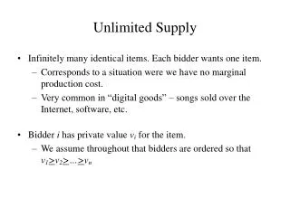
Unlimited Supply. Infinitely many identical items. Each bidder wants one item. Corresponds to a situation were we have no marginal production cost. Very common in “digital goods” – songs sold over the Internet, software, etc. Bidder i has private value v i for the item.

Unlimited Supply
E N D
Presentation Transcript
Unlimited Supply • Infinitely many identical items. Each bidder wants one item. • Corresponds to a situation were we have no marginal production cost. • Very common in “digital goods” – songs sold over the Internet, software, etc. • Bidder i has private value vi for the item. • We assume throughout that bidders are ordered so thatv1>v2>…>vn
Known probability distribution • If the values of the players are i.i.d from a probability distribution F, the we can use the optimal auction we already know: • Since we have unlimited supply, we need to determine, for every bidder separately, if she wins or loses. • So we need an optimal auction for one bidder. • We already know that this is a take-it-or-leave-it auction, with a reservation price p such that p=(1-F(p))/f(p)
Worst-case analysis • What if we do not know, and cannot estimate, the underlying probability distribution? • We will design an auction with revenue close to the following benchmark auction: • Suppose we know the values of the players, but must sell all items in the same price. The price will then be: F(v) = maxii·vi • Remark: a non-discriminatory monopoly chooses this price. • First attemp: find a small constant c and a truthful auction with revenue R(v) > F(v)/c for any input v. • Remark: this is called a worst-case analysis.
First difficulty • Reminder: a truthful auction must be monotone, and the price of a winner must be exactly her threshold value for winning. • Problem: suppose two players with v1=v2=1. Then F(v)=2. suppose we find a truthful auction with R(v)=2. • If we increase v1 to 100·c, 1’s price cannot change, so R(v)=2.=> R(v) < 100 = F(v)/c • Conclusion: situations with no competition are hopeless. • A fix: define F(2)(v) = maxi>2i·vi • For “most” cases F(v)= F(2)(v), and we want to avoid the extreme situations for which this is not true. • Second attempt: find a small constant c and a truthful auction with revenue R(v) > F(2)(v)/c for any input v.
A warm-up mechanism • Let A={1…n/2} and B={(n/2)+1,…,n} • Let pA and pB be the prices that achieve F(2)(v1,…,vn/2) and F(2)(vn/2+1,…,vn), respectively. • Each bidder i has a take-it-or-leave-it price:pA if iB and pB if iA. • Problem: suppose v1=v2=…=v50=2c >> 1, and v51=…=v100=1. What will happen? • pA = 2c and pB = 1. • Players 51..100 lose, and players 1,…50 win and pay $1 each • Overall R(v)=50 while F(2)(v)=50·2c, so R(v) < F(2)(v)/c
Allowing randomization • If the input contains 50 low bidders and 50 high bidders then “most” partitions will find the correct optimal price. The problem is that we deterministically chose one fixed partition. • A fix: allow the mechanism to toss coins. • Third (and final) attempt: find a small constant c and a truthful auction with expected revenue E[R(v)] > F(2)(v)/c for any v. • Remarks: • This is different than a randomization over the input v as we had up to now. In particular, we do not assume any known distribution. Instead, we create it. • Two truthfulness notions. Universal truthfulness: the auction is truthful for all coin tosses. Truthfulness-in-expectation: the player’s expected utility is maximized by being truthful.
A building block: truthful cost sharing • We want a revenue of exactly R (or cancel the entire auction). • The mechanism CostShare(R): collect bids b1,…,bn, and repeat: • Suppose we have k bids left (initially we have k=n). • If there exists a bid lower than R/k, delete it, and repeat. • Otherwise all remaining bidders win, and each one pays R/k. • Example: bids (5,4,3,2,1), R=9 • In the 1st round the tentative price is 9/5. Bid 5 is deleted. • In the 2nd round the tentative price is 9/4. Bid 4 is deleted. • In the 2nd round the tentative price is 9/3. All three remaining bids win, each one pays 9/3=3. Total revenue is 9.
A building block: truthful cost sharing Claim: • CostShare is truthful • The revenue is exactly R. Proof: left as exercise. • Observe that if F(v) > R then the item will indeed be sold, and the revenue will therefore be R.
Our auction • Randomly partition the bids to two sets (A, B) by tossing a fair coin for each player and associating her to A if the coin came out “head”, and otherwise to B. • Compute FA=F(A) and FB=F(B). • Run CostShare(A, FB) and CostShare(B, FA) to determine winners and prices. Claim: This auction is universally truthful proof: For every result of the coin toss, a player is associated to a fixed set (say A), and cannot affect FB. Therefore, truthfulness follows from the truthfulness of CostShare(A, FB)
Revenue Analysis (1) Claim: R(v) > min{F(A) , F(B)} Proof: • Suppose F(A) < F(B). • CostShare(B, F(B)) succeeds by definition • Therefore CostShare(B, F(A)) will also succeed, and will provide a profit of F(A).
A helpful fact • Flip a fair coin k>1 times. Let Ak,Bk denote the number of times it fell head,tail, respectively, and let Mk = min(Ak,Bk). Lemma: E[min(Ak,Bk)] > k/4.
A helpful fact • Flip a fair coin k>1 times. Let Ak,Bk denote the number of times it fell head,tail, respectively, and let Mk = min(Ak,Bk). Lemma: E[min(Ak,Bk)] > k/4. Proof: For any 1<i<k, define Xi = Mi – Mi-1 . Observe: • Mk = X1+…+Xk
A helpful fact • Flip a fair coin k>1 times. Let Ak,Bk denote the number of times it fell head,tail, respectively, and let Mk = min(Ak,Bk). Lemma: E[min(Ak,Bk)] > k/4. Proof: For any 1<i<k, define Xi = Mi – Mi-1 . Observe: • Mk = X1+…+Xk • for all i, Xi > 0=> E[Xi] > 0
A helpful fact • Flip a fair coin k>1 times. Let Ak,Bk denote the number of times it fell head,tail, respectively, and let Mk = min(Ak,Bk). Lemma: E[min(Ak,Bk)] > k/4. Proof: For any 1<i<k, define Xi = Mi – Mi-1 . Observe: • Mk = X1+…+Xk • for all i, Xi > 0=> E[Xi] > 0 • E[M2]=1/2 ; E[M3]=3/4 => E[X3]=E[M3]-E[M2]=1/4
A helpful fact • Flip a fair coin k>1 times. Let Ak,Bk denote the number of times it fell head,tail, respectively, and let Mk = min(Ak,Bk). Lemma: E[min(Ak,Bk)] > k/4. Proof: For any 1<i<k, define Xi = Mi – Mi-1 . Observe: • Mk = X1+…+Xk • for all i, Xi > 0=> E[Xi] > 0 • E[M2]=1/2 ; E[M3]=3/4 => E[X3]=E[M3]-E[M2]=1/4 • If i is even then E[Xi]=1/2: • i-1 is odd, so Ak ≠ Bk. Assume Ak > Bk . With prob. 1/2 the i’th coin is A and the minimun stays the same (so Xi=0) and with probability 1/2 it’s and the minimum increases by 1 (so Xi=1).
A helpful fact • Flip a fair coin k>1 times. Let Ak,Bk denote the number of times it fell head,tail, respectively, and let Mk = min(Ak,Bk). Lemma: E[min(Ak,Bk)] > k/4. Proof: For any 1<i<k, define Xi = Mi – Mi-1 . Observe: • Mk = X1+…+Xk • for all i, Xi > 0=> E[Xi] > 0 • E[M2]=1/2 ; E[M3]=3/4 => E[X3]=E[M3]-E[M2]=1/4 • If i is even then E[Xi]=1/2: • i-1 is odd, so Ak ≠ Bk. Assume Ak > Bk . With prob. 1/2 the i’th coin is A and the minimun stays the same (so Xi=0) and with probability 1/2 it’s and the minimum increases by 1 (so Xi=1). • E[Mk]=E[X1]+…+E[Xk] > 0 + 1/2 + 1/4 + 1/2 + 0 + 1/2 + 0 +…
A helpful fact • Flip a fair coin k>1 times. Let Ak,Bk denote the number of times it fell head,tail, respectively, and let Mk = min(Ak,Bk). Lemma: E[min(Ak,Bk)] > k/4. Proof: For any 1<i<k, define Xi = Mi – Mi-1 . Observe: • Mk = X1+…+Xk • for all i, Xi > 0=> E[Xi] > 0 • E[M2]=1/2 ; E[M3]=3/4 => E[X3]=E[M3]-E[M2]=1/4 • If i is even then E[Xi]=1/2: • i-1 is odd, so Ak ≠ Bk. Assume Ak > Bk . With prob. 1/2 the i’th coin is A and the minimun stays the same (so Xi=0) and with probability 1/2 it’s and the minimum increases by 1 (so Xi=1). • E[Mk]=E[X1]+…+E[Xk] > 0 + 1/2 + 1/4 + 1/2 + 0 + 1/2 + 0 +… = =1/4 + (k/2)·(1/2) > 1/4 + (k-1)/4 = k/4.
Revenue Analysis (2) Lemma: E[R(v)] > F(2)(v)/4 Proof: • Recall that R(v) > min{F(2)(A) , F(2)(B)} • Suppose F(2)(v) = y·p (p is the monopolistic price). • Let yA,yB denote the number of bids larger than p that belong to A,B, respectively. Note that y= yA+yB. • Observe that F(A) > yA·p , F(B) > yB·p E[R(v)] > E[min{F(A) , F(B)}] > E[min{yA·p , yB·p}] == p·E[min{yA , yB}] > p·y/4 = F(2)(v)/4.
Remarks • The factor c is called the “approximation factor” (or approximation ratio). This is a notion from computer science. • The best approximation factor known for this setting is 3.25. It is also known that no truthful auction can approximation factor better than 2.42.
Bibliographic notes • Worst-case analysis is the standard in computer science (as opposed to all other sciences…) • This work indeed came from computer scientists (Fiat, Goldberg, Hartline, and Karlin, 2002). • The interaction of CS and Economics is quite new, and it is not clear what performs better in practice • Designing an auction based on distributional knowledge we don’t have (and then estimating it somehow), or • Designing a worst-case auction that gives worst-case bounds (that are of-course lower than the bounds of above). • In particular, an experimental study that evaluates this would be interesting and useful.