Download

1 / 29
290 likes | 406 Vues
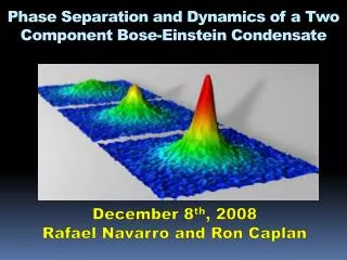
Phase Separation and Dynamics of a Two Component Bose-Einstein Condensate. December 8 th , 2008 Rafael Navarro and Ron Caplan. Overview. Purpose of Study Introduction to BECs Mean-field model for coupled BEC Variational Approach and Reduction to System of ODEs

E N D
Phase Separation and Dynamics of a Two Component Bose-Einstein Condensate December 8th, 2008 Rafael Navarro and Ron Caplan
Overview • Purpose of Study • Introduction to BECs • Mean-field model for coupled BEC • Variational Approach and Reduction to System of ODEs • Introduction to Continuous Dynamical Systems. • Steady states of reduced model, and Bifurcations of parameters. • Further reduction of the system to a Newton style Equation, its bifurcations, and comparison of dynamics. • Conclusion.
Purpose • The goal of this work is to attain a global description of how two condensates different spin interact with each other. • We wish to give a criteria for miscibility (mixing) and frequency of oscillation between the two condensates. • Also, the stability of the system is studied.
Introduction to BEC De Broglie: All particles are wave-like, with wavelength depended on momentum. Heisenberg: Uncertainty in momentum and position related: x p = h In a gas, there is an average distance between atoms called the scattering length, d. x p= h xp= h x p = h
Properties of a BEC • In BECs, bosons occupy the same quantum mechanical ground state. • All atoms in the BEC act as one and move in unison. • The condensate displays wave properties which can be modeled using the Nonlinear Schrödinger Equation (NLS). • Two component BECs are when two sets of atoms, each in a different spin state are formed into a BEC together. They interact with each other, and typically repel each other. • The dynamics of a two-component BEC can be modeled using two coupled NLS equations.
BEC in a Quasi 1-D trap • The external is generated by a magnetic trap and is very narrow in the transverse direction x< y=z. • The system is quasi 1-dimensional and two degrees of freedom can be integrated out of the NLS.
Coupled Nonlinear Schrodinger Equations (NLS) Time Dependence Term Kinetic Energy Term External Potential Term Interaction Term: Like Species Interaction Term: Unlike Species Species #1 Species #2 Wave Function Atom’s Mass Coupling Constant Between Species 2 and 2 Coupling Constant Between Species 2 and 1 Plank’s Constant Atomic Density
Renormalized Equations By rescaling time, space, the wave function, and coupling constant, we can undimensionalize the system and get:
Variational Model • The Lagrangian is a functional that represents the energy of the system. • When the variation of the Lagrangian is minimized, the optimum solution is obtained. L1 = Lagrangian of first species L2 = Lagrangian second species L12 = Interaction LagrangianE = Mechanical energy of system
Wave Packet Trial Function • We propose a wave-packet trial function composed of a carrier wave packet. • The wave packet has amplitude A, position B, width W, phase C, frequency D, and frequency modulation E.
Euler-Lagrange Equations • The Lagrangian is evaluated for the trial function yielding: • Equations of motion (ODEs) can be obtained for each parameter of the trial function through the Euler Lagrange equations • p1= A, p2= B, p3= C, p4= D, p5= E, p6= W.
Analogy to Lorenz Equation . • Lorentz’s system of three coupled nonlinear ordinary differential equations were obtained by approximating the Navier-Stokes equations, a set of five coupled partial differential equations. • In our case, we used the VA to obtainODEs describing the motion of our solution form the system of PDEs
Continuous Dynamical Systems • The system can be linearized by (J is called the Jacobian of the system.) • A fixed point is stable when real(i)<0, for all i=1,2,…,n and unstable otherwise. Here, i represents the eigenvalues of J. • Note the difference here compared to discrete dynamics - that our critical eigenvalue is 0 rather than 1 • The fixed points, p*, on continuous dynamical system are obtained by:
Phase Portraits In a system of ODEs, we can plot the orbits on a phase portrait We plot a arrow-field which shows the direction that an orbit will take. As an example, we look at different possibilities in a 2-dimentional system (J2x2):
Fixed Points of our System • Mixed State Fixed Points: • Separated State Fixed Points:
Trial Function Matches Full Solution Separated State Mixed State
Bifurcation of Position, B D = supercritical pitchfork bifurcation points A = transcritical pitchfork bifurcation points B = saddle node bifurcation points
Dynamics of Mixed State PDE (solid line)ODE (dashed line)
Dynamics of Separated State PDE (solid line)ODE (dashed line)
Reduced Dynamics • It is possible to obtain a simple equation for the dynamics of the position of the condensate. • If we assume that the variations in the amplitude and width are small, the time dependent amplitude and width can be replaced by the steady state amplitude and width: A(t)A* and B(t) B*. • The motion can be described in terms of a potential, Ueff. • Ueff = (atom-atom interaction) + (atom-potential interaction)
Three Orbits: • Potential Function • Phase Portrait • Position vs. Time
Conclusion • We have shown the reduction of a coupled system of PDEs into a system of ODEs using the variational approach with a trial function. • We performed stability analysis on the steady state solutions to the system of ODEs. • We found bifurcations and stability of different parameters, and found miscibility conditions. • The point of phase transition is predicted well by the reduced model, but the equilibrium value of the parameters near the phase transition point deviate from the PDE’s solution. • We then reduced the model to a Newton-style equation and numerically compared the reduced model, the system of ODEs and the PDEs and showed that generally, the ODEs and Newton equations are very good at describing the dynamics of the system for fully separated states and fully mixed states.