Download
1 / 23
230 likes | 406 Vues
Lecture #21 EGR 270 – Fundamentals of Computer Engineering. Reading Assignment: Chapter 6 in Logic and Computer Design Fundamentals 4 th Edition by Mano. The Design Space For a given design, there is typically:

E N D
Lecture #21 EGR 270 – Fundamentals of Computer Engineering Reading Assignment: Chapter 6 in Logic and Computer Design Fundamentals 4th Edition by Mano • The Design Space • For a given design, there is typically: • a target implementation technology (i.e., a logic family) that specifies the primitive elements available and the properties of those elements. • a set of constraints that applies to the design • We will now discuss some of the primitive gate properties and design constraint tradeoffs. • Levels of integration – the following terms are sometimes used to describe packages by • indicating whether their implementation requires just a few gates or millions. • SSI: Small-scale integration - equivalent of 1 - 9 gates • MSI: Medium-scale integration - equivalent of 10 - 100 gates • Examples: Decoders, encoders, multiplexers, adders • LSI: Large-scale integration - between 100 and a few thousand gates • Examples: Small memory chips or processors, programmable modules • VLSI: Very large-scale integration - several thousand to tens of millions of gates • Examples: Complex microprocessors, digital signal processing (DSP) chips • Because of their high density and low cost, VLSI devices have revolutionized • digital system and computer design.
Lecture #21 EGR 270 – Fundamentals of Computer Engineering • Circuit Technologies • Logic circuits can be implemented using several technologies, each of which have • different characteristics. Logic families include: • TTL (transistor-transistor technology) • Older technology, but works well for small projects, lab experiments, etc. • Sub families include standard TTL (7400 series), low-power Shottkey TTL (74LS00 series), etc. Not static sensitive. • CMOS (Complementary Metal Oxide Semiconductor) • Dominant technology due to high circuit density, high performance, and low power consumption. Static sensitive. • GaAs (Gallium Arsenide) and SiGe (Silicon Germanium) • Used in some selective very high speed applications. • Others
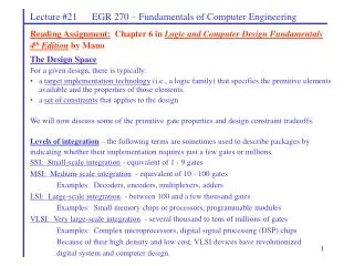
Figure 3-5: Implementation of a 7-input NAND gate using NAND gates with 4 or fewer inputs. Lecture #21 EGR 270 – Fundamentals of Computer Engineering • Technology Parameters (logic circuit properties) – the following parameters are • Used to characterize each implementation technology (or logic family): • Fan-in • Propagation delay • Fan-out • Noise margin – the maximum amount of noise voltage allowed such that the valid output of one gate will still yield a valid input. • Cost – related to the area occupied by the circuit • Power dissipation – power drawn from the power supply and dissipated by the gate. Note that power consumed by a gate is dissipated as heat. • Fan-In • Fan-in specifies the number of inputs available on a gate. • Gate primitives in HDL often limit the number of inputs to 4 or 5. • To build gates with lower fan-in, multiple gates can be interconnected.
Lecture #21 EGR 270 – Fundamentals of Computer Engineering • Propagation Delay • When changes to a gate’s input result in the output changing logic levels, a certain amount of time is required for the change to take place. This time delay is referred to as propagation delay. • Three specifications for propagation delay are typically used: • tPHL = delay in the output changing from HIGH to LOW • tPLH = delay in the output changing from LOW to HIGH • tpd = maximum of tPHL and tPLH • Propagation delay is illustrated for an inverter in Figure 3-6 below. Note that the waveforms do not change instantly from L to H or from H to L. So where is the propagation delay measured? • Propagation delay is measured at the 50% point in each waveform.
Lecture #21 EGR 270 – Fundamentals of Computer Engineering • Fan-Out for TTL gates • Fan-out specifies the number of standard loads that can be driven by a gate output. • Standard loads are defined differently for different technologies. • In TTL, a standard load is simply an input to another gate. • In TTL, fan-out is primarily a function of current. • For example, if the LOW output of a TTL gate can provide up to 16mA and if the LOW input to a TTL gate can require up to 1.6mA, then the fan-out is 16mA/1.6mA = 10, or 10 standard loads can be driven by the output of one gate. • Note that we are more concerned with CMOS technology than TTL (next page!)
Lecture #21 EGR 270 – Fundamentals of Computer Engineering • Fan-Out for CMOS gates • Fan-out specifies the number of standard loads that can be driven by a gate output. • Standard loads are defined differently for different technologies. • CMOS gates require almost no input current, but loads act like capacitance which slows the gate’s response. • The inputs to CMOS gates provide loads that are measured in “standard load units”. Table 3-3 provided on the following page shows standard load units for various gates. • Table 3-3 indicates that propagation delay can be calculated as follows: • tpd = unloaded value + constant*SL (in ns), where SL = number of standard loads • For example, an inverter has the following delay: tpd = 0.04 + 0.012*SL ns • Note that additional delay can be caused by capacitance between wires in a circuit. • Example: Find the propagation delay for the 4-input NAND in the following circuit:
Lecture #21 EGR 270 Table 3-3 Example Cell Library for Technology Mapping Note: Normalized area is used as “cost” in text examples
Lecture #21 EGR 270 – Fundamentals of Computer Engineering • Design Tradeoffs • Tradeoffs can occur when designing a circuit, such as the area a circuit occupies (cost) versus the propagation delay (performance). • Cost/performance tradeoffs are the most common type of tradeoff. • A given design may need to satisfy various constraints and tradeoffs may need to be considered to satisfy the constraints. • Example: • Consider the two cases below. • Case 1: Gate G driving 16 standard loads has tpd = 0.406 ns. Gate G has a cost of 2.0 • Case 2: Gate G driving only a buffer connected to the 16 standard loads has a delay of 0.323 ns. Gate G plus the buffer have a cost of 3.0. • So the delay is reduced, but the cost is increased. Which is best? • It may depend on constraints: • If we have a constraint that tpd(max) = 0.35ns, then Case 2 would be selected. • If we have a constraint that the max area to be used is 2.5, then Case 1 would be selected.
X Z F(X,Y,Z) = (3,4,6,7) = XZ’ + YZ X Y 1 1 Y 1 1 Z 0 1 F Glitch Lecture #21 EGR 270 – Fundamentals of Computer Engineering Example: Note that for the following logic circuit, F = 1 for inputs 3, 4, 6, and 7. However, when the input changes from 7 to 6 a glitch occurs (we will see why shortly). Timing Hazards * So far we have ignored circuit delay in combinational logic circuits. Our circuits produce the correct outputs if their inputs have been stable for a long time (i.e., in steady-state). However, their transient behavior may differ from their steady state behavior. In particular, the circuit’s output may produce a short pulse, or “glitch” , due to uneven delays in different signal paths. Hazard – a circuit is said to have a hazard when it has the possibility of producing a glitch. The glitch may only occur after the transition between certain combinations of inputs. The designer of a logic circuit should be prepared to eliminate hazards (the possibility of glitches). * Reference: Digital Design – Principles and Practices, 3rd Edition by John Wakerly, Prentice-Hall, 2002.
Glitch due to a static-1 hazard Glitch due to a static-0 hazard Logic Circuit Input Output Lecture #21 EGR 270 – Fundamentals of Computer Engineering Types of hazards 1) Static hazards – A static hazard is a hazard where the output should have a stable (static) value, but a glitch may occur briefly producing the opposite logic value. There are two types of static hazards: A) Static-1 Hazard – the circuit has the possibility of producing an unwanted 0 glitch. B) Static-0 Hazard – the circuit has the possibility of producing an unwanted 0 glitch. 2) Dynamic hazards – The possibility of an output changing more than once as the result of a single input transition. Multiple output transitions can occur if there are multiple paths with different delays from the changing input to the changing output. Example: Dynamic hazard 10 Input waveform Output waveform
Glitch due to a static-1 hazard Lecture #21 EGR 270 – Fundamentals of Computer Engineering Static-1 Hazards A static-1 hazard is the possibility of a circuit producing a 0 glitch when we would expect the circuit to remain a steady logic 1. Definition: A static-1 hazard is a pair of input combinations that a) differ in only one input variable and b) both give an output 1 (i.e., adjacent minterms in a K-map); such that it is possible for a momentary 0 output to occur during a transition in the differing input variable. A K- map can be used to detect static hazards in a two-level SOP circuit. Groupings of 1’s in K-maps correspond to product terms (AND gates) in SOP expressions. If an output of 1 is produced by one product term and then a change in input produces a 1 by an adjacent product, then there is the possibility of a glitch where the output momentarily goes to logic 0. The hazard can be eliminated by adding an additional product term which overlaps the existing two product terms. The extra product term is the consensus of the original two terms. * In general, we must add consensus terms to eliminate hazards. 11
BC A 00 01 11 10 1 0 1 1 1 Lecture #21 EGR 270 – Fundamentals of Computer Engineering Example: Static-1 Hazard A minimal Sum of Products (SOP) expression of the function F(A,B,C) = (3,4,6,7) can be found using a Karnaugh map as follows: The resulting expression is: F1(A,B,C) = AC’ + BC (minimal SOP) 1 Problem: The circuit has a static-1 hazard. In particular, the output should remain HIGH as the input changes from input m7 to m6, but it actually goes briefly LOW. A Input changes from m7 (111) to m6 (110) B C F1 Glitch (static-1 hazard)
BC A 00 01 11 10 1 0 1 1 1 Lecture #21 EGR 270 – Fundamentals of Computer Engineering Solution: This problem can be corrected by adding a “consensus term”. m6 is covered by the product term AC’ and m7 is covered by the product term BC. The term AC’ has additional propagation delay since C is inverted, resulting in a “glitch” in the output. The consensus term AB overlaps the other two product terms and eliminates the glitch. The new Karnaugh map is shown below: The resulting expression after adding the consensus term is: F2(A,B,C) = AC’ + BC + AB (static-1 hazard eliminated) 1
Lecture #21 EGR 270 – Fundamentals of Computer Engineering Timing Diagram: Show that F1 contains a static-1 hazard and that F2 does not. F1(A,B,C) = AC’ + BC- should contain a glitch as the input changes from m7 to m6 F2(A,B,C) = AC’ + BC + AB - glitch should be removed A B C BC C’ AC’ F1 AB F2
Lecture #21 EGR 270 – Fundamentals of Computer Engineering PSPICE Simulation Digital Clocks are used in PSPICE in the example below to apply the inputs XYZ from 111 to 000. The inputs are applied to the original circuit containing a static-1 hazard (output F1) and the corrected circuit (output F2). The timing diagram on the following pages shows that the hazard was successfully removed.
Static-1 Hazard Lecture #21 EGR 270 – Fundamentals of Computer Engineering F1 = XZ’ + YZ = output of original circuit with static-1 hazard F2 = XZ’ + YZ + XY = output of corrected circuit (hazard eliminated)
Glitch due to a static-0 hazard Lecture #21 EGR 270 – Fundamentals of Computer Engineering Static-0 Hazards A static-0 hazard is the possibility of a circuit producing a 1 glitch when we would expect the circuit to remain a steady logic 0. Definition: A static-0 hazard is a pair of input combinations that a) differ in only one input variable and b) both give an output 0 (i.e., adjacent maxterms in a K-map); such that it is possible for a momentary 1 output to occur during a transition in the differing input variable. A K- map can be used to detect static hazards in a two-level POS circuit. Groupings of 0’s in K-maps correspond to sum terms (OR gates) in POS expressions. If an output of 0 is produced by one sum term and then a change in input produces a 0 by an adjacent sum term, then there is the possibility of a glitch where the output momentarily goes to logic 1. The hazard can be eliminated by adding an additional sum term which overlaps the existing two sum terms. The extra sum term is the consensus of the original two terms. * In general, we must add consensus terms to eliminate hazards. 17
Lecture #21 EGR 270 – Fundamentals of Computer Engineering Example: Static-0 Hazard A minimal Product of Sums (POS) expression of the function F(A,B,C) = (0,1,3,4) = (2,5,6,7) can be found using a K- map as follows: BC A 00 01 11 10 0 0 0 1 The resulting expression is: F1’(A,B,C) = B’C’ + A’C F1(A,B,C) = (B+C)(A+C’) (minimal POS) 0 1 0 1 1 1 Problem: The circuit has a static-0 hazard. In particular, the output should remain LOW as the input changes from input m0 to m1, but it actually goes briefly HIGH. A Input changes from m0 (000) to m1 (001) B C F1 18 Glitch (static-0 hazard)
BC A 00 01 11 10 0 1 Lecture #21 EGR 270 – Fundamentals of Computer Engineering Solution: This problem can be corrected by adding a “consensus term”. m0 is covered by the product term B’C’ and m1 is covered by the product term A’C. The term A’C has additional propagation delay since C is inverted (after applying DeMorgan’s theorem to form F2 from F2’), resulting in a “glitch” in the output. The consensus term A’B’ overlaps the other two product terms and eliminates the glitch. The new Karnaugh map is shown below: The resulting expression after adding the consensus term is: F2’(A,B,C) = B’C’ + A’C + A’B’ F2(A,B,C) = (B+C)(A+C’)(A+B) (static-0 hazard eliminated) 0 0 0 1 0 1 1 1
Lecture #21 EGR 270 – Fundamentals of Computer Engineering Timing Diagram: Show that F1 contains a static-0 hazard and that F2 does not. F1(A,B,C) = (B+C)(A+C’) - should contain a glitch as the input changes from m0 to m1 F2(A,B,C) = (B+C)(A+C’)(A+B) - glitch should be removed A B C B+C C’ A+C’ F1 A+B F2
Lecture #21 EGR 270 – Fundamentals of Computer Engineering Note: Circuits may contain multiple hazards. In general, all possible consensus terms should be added to eliminate the possibility of glitches. Example: Redesign the function F(A,B,C,D) = A’B + AC + B’C’D to eliminate all static-1 hazards. Draw a timing diagram to illustrate one input transition where a glitch could occur.
Lecture #21 EGR 270 – Fundamentals of Computer Engineering Flip-flop timing When propagation delay was introduced earlier in the course, the terms tpHL, tpLH, and tpd were introduced and worked well to describe the delays encountered in combinational logic gates. Other terms are sometimes used when dealing with flip-flops: ts – setup time for which the flip-flop inputs (S, R, D, etc) must be maintained as constant values prior to the clock occurrence that causes the output to change. th – hold time for which the flip-flop inputs (S, R, D, etc) must be maintained as constant values after the clock occurrence that causes the output to change (so that the master can transfer the data to the slave). tw – clock pulse width . Note that there is a minimum value of tw for the master to capture the input values correctly. Note that ts typically is smaller for edge-triggered devices, so edge-triggered devices typically provide for faster designs that pulse-triggered devices. tpHL, tpLH, and tpd – are defined as the interval between the triggering clock edge and the stabilization of the output to a new value. Figure 6-16 from the text (shown on the next page) illustrates these delays.
Lecture #21 EGR 270 – Fundamentals of Computer Engineering