Download

1 / 113
1.13k likes | 1.17k Vues
Discover the intricacies of Chaos Theory and Nonlinear Dynamics, where small changes lead to vastly different outcomes in complex systems. Learn about N-body problems, pioneering figures like Jules Henri Poincarè, and the concept of chaotic behavior in science. Explore the impact of Chaos Theory on deterministic predictions and the fascinating world of dynamical systems. Uncover how chaos and order coexist in a system's evolution, and the significance of state space in understanding complex dynamics.

E N D
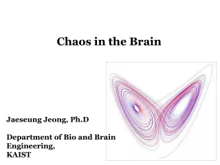
Chaos in the Brain Jaeseung Jeong, Ph.D Department of Bio and BrainEngineering, KAIST
Nonlinear dynamics and Chaos : the tiniestchange in the initial conditions produces a very different outcome, even when the governing equations are known exactly - neither predictable nor repeatable Chaos 1. the formless shape of matter that is alleged to have existed before the Universe was given order. 2. complete confusion or disorder. 3. Physics;a state of disorder and irregularity that is an intermediate stage between highly ordered motion and entirely random motion.
Nonlinear dynamics and Chaos (2) King Oscar II (1829 – 1907) offered a prize of 2500 crowns to anyone solve the n-body problem stability of the Solar System
Nonlinear dynamics and Chaos • N-body problem The classical n-body problem is that given the initial positions and velocities of a certain number (n) of objects that attract one another by gravity, one has to determine their configuration at any time in the future..
Nonlinear dynamics and Chaos (3) Jules Henri Poincarè (1854 – 1912) Won the Oscar II’s contest, not for solving the problem, but for showing that even the three-body problem was impossible to solve. (over 200 pages ) “…it may happen that small differences in the initial conditions produce very great ones in the final phenomena. A small error in the former will produce an enormous error in the latter. Prediction becomes impossible, and we have the fortuitous phenomenon” - in a 1903, essay "Science and Method"
Nonlinear dynamics and Chaos • N-body problem This problem arose due to a deterministic way of thought, in which people thought they could predict into the future provided they are given sufficient information. However, this turned out to be false, as demonstrated by Chaos Theory.
Nonlinear dynamics and Chaos Systems behaving in this manner are now called “chaotic.” They are essentially nonlinear, indicating that initial errors in measurements do not remain constant, rather they grow and decay nonlinearly (usually exponentially) with time. Since prediction becomes impossible, these systems can appear to be irregular, but this randomness is only apparent because the origin of their irregularities is different: they are intrinsic, rather than due to external influences.
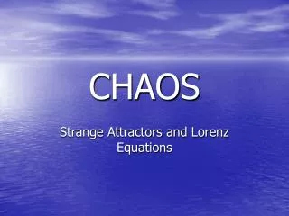
What is chaos? • The meteorologist E. Lorenz He modeled atmospheric convection in terms of three differential equations and described their extreme sensitivity to the starting values used for their calculations. • The meteorologist R May He showed that even simple systems (in this case interacting populations) could display very “complicated and disordered” behavior. • D. Ruelle and F. Takens They related the still mysterious turbulence of fluids to chaos and were the first to use the name ‘strange attractors.’
Nonlinear dynamics and Chaos Lorenz attractor
The Logistic equation • Xn+1=AXn(1-Xn)
Nonlinear dynamics and Chaos • Laminar(regular) / Turbulent(chaotic) • Turbulent of gas flows
Nonlinear dynamics and Chaos • High flow rate: Laminar Turbulent Department of BioSystems
What is Chaos? • M Feigenbaum He revealed patterns in chaotic behavior by showing how the quadratic map switches from one state to another via periodic doubling. • TY Li and J Yorke They introduced the term ‘chaos’ during their analysis of the same map. • A. Kolmogorov and YG Sinai They characterized the properties of chaos and its relations with probabilistic laws and information theory.
Nonlinear dynamics and Chaos • Taffy – pulling machine
Nonlinear dynamics and Chaos • The strength of science It lies in its ability to trace causal relations and so to predict future events. • Newtonian Physics Once the laws of gravity were known, it became possible to anticipate accurately eclipses thousand years in advance. • Determinism is predictability The fate of a deterministic system is predictable • This equivalence arose from a mathematical truth: Deterministic systems are specified by differential equations that make no reference to chance and follow a unique path.
Chaos systems • Newtonian deterministic systems (Deterministic, Predictable) • Probabilistic systems (Non-deterministic, Unpredictable) • Chaotic systems (Deterministic, Unpredictable)
Dynamical system and State space • A dynamical system is a model that determines the evolution of a system given only the initial state, which implies that these systems posses memory. • The state space is a mathematical and abstract construct, with orthogonal coordinate directions representing each of the variables needed to specify the instantaneous stae of the system such as velocity and position • Plotting the numerical values of all the variables at a given time provides a description of the state of the system at that time. Its dynamics or evolution is indicated by tracing a path, or trajectory, in that same space. • A remarkable feature of the phase space is its ability to represent a complex behavior in a geometric and therefore comprehensible form (Faure and Korn, 2001).
For any phenomena, they can all be modeled as a system governed by a consistent set of laws that determine the evolution over time, i.e. the dynamics of the systems.
Linear vs. NonlinearConservative vs. DissipativeDeterministic vs. Stochastic • A dynamical system is linear if all the equations describing its dynamics are linear; otherwise it is nonlinear. • In a linear system, there is a linear relation between causes and effects (small causes have small effects); in a nonlinear system this is not necessarily so: small causes may have large effects. • A dynamical system is conservative if the important quantities of the system (energy, heat, voltage) are preserved over time; if they are not (for instance if energy is exchanged with the surroundings) the system is dissipative. • Finally a dynamical system is deterministic if the equations of motion do not contain any noise terms and stochastic otherwise.
Attractors • A crucial property of dissipative deterministic dynamical systems is that, if we observe the system for a sufficiently long time, the trajectory will converge to a subspace of the total state space. This subspace is a geometrical object which is called the attractor of the system. • Four different types of Attractors: • Point attractor: such a system will converge to a steady state after which no further changes occur. • Limit cycle attractors are closed loops in the state space of the system: period dynamics. • Torus attractors have a more complex ‘donut like’ shape, and correspond to quasi periodic dynamics: a superposition of different periodic dynamics with incommensurable frequencies (Faure and Korn, 2001; Stam 2005).
Chaotic attractors • The chaotic (or strange) attractor is a very complex object with a so-called fractal geometry. The dynamics corresponding to a strange attractor is deterministic chaos. • Chaotic dynamics can only be predicted for short time periods. • A chaotic system, although its dynamics is confined to the attractor, never repeats the same state. • What should have become clear from this description is that attractors are very important objects since they give us an image or a ‘picture’ of the systems dynamics; the more complex the attractor, the more complex the corresponding dynamics.
Characterization of the attractors I • If we take an attractor and arbitrary planes which cuts the attractor into two pieces (Poincaré sections), the orbits which comprise the attractor cross the plane many times. • If we plot the intersections of the orbits and the Poincaré sections, we can know the structure of the attractor.
Characterization of the attractors II • The dimension of a geometric object is a measure of its spatial extensiveness. The dimension of an attractor can be thought of as a measure of the degrees of freedom or the ‘complexity’ of the dynamics. • A point attractor has dimension zero, a limit cycle dimension one, a torus has an integer dimension corresponding to the number of superimposed periodic oscillations, and a strange attractor has a fractal dimension. • A fractal dimension is a non integer number, for instance 2.16, which reflects the complex, fractal geometry of the strange attractor.
Characterization of the attractors III • Lyapunov exponents can be considered ‘dynamic’ measures of attractor complexity. • Lyapunov exponents indicate the exponential divergence (positive exponents) or convergence (negative exponents) of nearby trajectories on the attractor. • A system has as many Lyapunov exponents as there are directions in state space.
Characterization of the attractors IV • A chaotic system can be considered as a source of information: it makes prediction uncertain due to the sensitive dependence on initial conditions. • Any imprecision in our knowledge of the state is magnified as time goes by. A measurement made at a later time provides additional information about the initial condition. • Entropy is a thermodynamic quantity describing the amount of disorders in a system.
Control parameters and multistability • Control parameters are those system properties that can influence the dynamics of the system and that are either held constant or assumed constant during the time the system is observed. • Parameters should not be confused with variables, since variables are not held constant but are allowed to change. • Multistability: For a fixed set of control parameters, a dynamical system may have more than one attractor. • Each attractor occupies its own region in the state space of the system. Surrounding each attractor there is a region of state space called the basin of attraction of that attractor. • If the initial state of the system falls within the basin of a certain attractor, the dynamics of the system will evolve to that attractor and stay there. Thus in a system with multi stability the basins will determine which attractor the system will end on.
Bifurcations • In a multistable system, the total of coexisting attractors and their basins can be said to form an ‘attractor landscape’ which is characteristic for a set of values of the control parameters. • If the control parameters are changed this may result in a smooth deformation of the attractor landscape. • However, for critical values of the control parameters the shape of the attractor landscape may change suddenly and dramatically. At such transitions, called bifurcations, old attractors may disappear and new attractors may appear (Faure and Korn, 2001; Stam 2005).
This EEG time series shows the transition between interictal and ictal brain dynamics. The attractor corresponding to the inter ictal state is high dimensional and reflects a low level of synchronization in the underlying neuronal networks, whereas the attractor reconstructed from the ictal part on the right shows a clearly recognizable structure. (Stam, 2003)
Route to Chaos • Period doubling As the parameter increases, the period doubles: period-doubling cascade, culminating into a behavior that becomes finally chaotic, i.e. apparently indistinguishable visually from a random process • Intermittency A periodic signal is interrupted by random bursts occurring unpredictably but with increasing frequency as a parameter is modified. • Quasiperiodicity A torus becomes a strange attractor.
Detecting chaos in experimental data • Bottom-up approach We can apply nonlinear dynamical system methods to the dynamical equations, if we know the set of equations governing the basic systems variables. • Top-down approach • However, the starting point of any investigation in experiments is usually not a set of differential equations, but rather a set of observations. • The way to get from the observations of a system with unknown properties to a better understanding of the dynamics of the underlying system is nonlinear time series analysis. • Starting with the output of the system, and working back to the state space, attractors and their properties.
General strategy of nonlinear dynamical analysis • Nonlinear time series analysis is a procedure that consists of three main steps: • (i) reconstruction of the system’s dynamics in the state space using delay coordinates and embedding procedure. • (ii) characterization of the reconstructed attractor using various nonlinear measures • (iii) checking the validity (at least to a certain extent) of the procedure using the surrogate data methods.
Reconstruction of system dynamics [problem] our measurements usually do not have a one to one correspondence with the system variables we are interested in. For instance, the actual state space may be determined by ten variables of interest, while we have only two time series of measurements; each of these time series might then be due to some unknown mixing of the true system variables.
Delay coordinate and Embedding procedure • With embedding, one time series are converted to a series or sequence of vectors in an m-dimensional embedding space. • If the system from which the measurements were taken has an attractor, and if the embedding dimension m is sufficiently high, the series of reconstructed vectors constitute an ‘equivalent attractor’ (Whitney, 1936). • Takens has proven that this equivalent attractor has the same dynamical properties (dimension, Lyapunov spectrum, entropy etc.) as the true attractor (Takens, 1981). • We can obtain valuable information about the dynamics of the system, even if we don't have direct access to all the systems variables.
Takens’ Embedding theorem (1981) Takens has shown that, if we measure any single variable with sufficient accuracy for a long period of time, it is possible to reconstruct the underlying dynamic structure of the entire system from the behavior of that single variable using delay coordinates and the embedding procedure.
Time-delay embedding • We start with a single time series of observations. From this we reconstruct the m-dimensional vectors by taking m consecutive values of the time series as the values for the m coordinates of the vector. • By repeating this procedure for the next m values of the time series we obtain the series of vectors in the state space of the system. • The connection between successive vectors defines the trajectory of the system. In practice, we do not use values of the time series of consecutive digitizing steps, but use values separated by a small ‘time delay’ d.
Parameter choice • Time delay d: a pragmatic approach is to choose l equal to the time interval after which the autocorrelation function (or the mutual information) of the time series has dropped to 1/e of its initial value. • Embedding dimension m: repeat the analysis (for instance, computation of the correlation dimension) for increasing values of m until the results no longer change; one assumes that is the point where m>2d (with d the true dimension of the attractor).