Download
1 / 36
360 likes | 382 Vues
Learn about Nash equilibrium, pure and mixed strategies, strategic uncertainty, and competition strategies in economics and game theory.

E N D
Lecture 4Nash Equilibrium andStrategic Uncertainty In some games even iterative dominance does not help us predict what strategies players might choose. For that reason, we relax the criteria a solution should satisfy, by introducing the concept of a Nash equilibrium. We analyze both pure and mixed strategy Nash equilibrium. This leads into to a discussion of strategic uncertainty, uncertainty collectively but non-cooperatively induced by the players rather than the information technology.
Motivation for Nash equilibrium • After eliminating iteratively dominated strategies, we are sometimes left with many possible strategic profiles. • In these cases we must impose more stringent assumptions on how players behave to reach a sharper prediction about the outcome of a game. • As before suppose you do not have data to estimate the probability distribution of the choices by the other players. One approach is to form a conjecture about the other players’ strategies, and then maximizes your payoffs subject to this conjecture. • This in essence describes our motivation for resorting to the concept of a Nash equilibrium.
The Nash equilibrium concept • The concept of a Nash equilibrium applies to the strategic form of a game, not its extensive form. • Suppose every player forms a conjecture about the choices of other players, and then chooses his best reply to that conjecture. • After every player has moved in this way each one observes the choices of all the other players. • Their collective choices constitute a Nash equilibrium if none of the conjectures by any player was contradicted by the choice of another player.
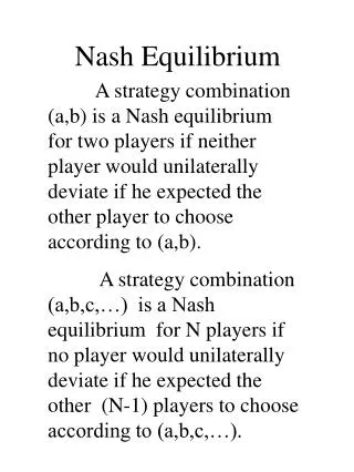
Definition of a Nash equilibrium • Consider an N player finite game, where sn is the strategy of the nth player where 16 n6 N. • Also write s-n for the strategy of every player apart from player n. That is: s-n = (s1, . . ., sn-1, sn+1, . . ., sN). • Now ask whether sn is the best response of n to s-n for all n? If so, nobody has an incentive to unilaterally deviate from their assigned strategy. • This is called a Nash equilibrium.
Dominance solvable games • In the celebrated game of the prisoners’ dilemma, both players have dominant strategies to confess. • We illustrate the best response with vertical arrows for the row player and horizontal arrows for the column player. • A Nash equilibrium occurs where there is neither a vertical nor a horizontal arrow pointing out of the box. • Thus if each player has a dominant strategy, then the solution to the Prisoner’s dilemma game is a Nash equilibrium.
Nash equilibrium encompasses iterated dominance (and backwards induction) • More generally the solution to every dominance game is a Nash equilibrium. • We prove that if sn is not a best response for every player n, it is not the solution to a dominance solvable game. The details of the proof are on the next slide. • Suppose that contrary to the claim sn is not a best response. That means the best response is some other strategy rn. • Then we show that sn cannot iteratively dominate at least one other strategy, and therefore is not part of a dominance solvable solution.
Proof • Note a solution sn derived from iterative dominance is a best response by every player to the reduced game after a finite number of strategies have been eliminated. • Suppose sn is not a best reply. Then there exists an eliminated strategy called rn that yields a strictly higher payoff to player n than the solution strategy sn. • Consequently rn is not dominated by sn. Since it was eliminated, it must be iteratively dominated by another strategy rn’ and hence rn’ also gives a higher yield than sn. • By induction sn cannot iteratively dominate those strategies that iteratively dominate rn. • Thus sn cannot be part of the solution to this dominance solvable game if it is not a best reply.
Competition through integration • In this game, a specialized producer of components for a durable good has the option of integrating all the way down to forming dealership, but indirectly faces competition from a retailer, which markets similar final products, possibly including the supplier’s.
Retailer • The profits of the retailer on this item fall the more integrated is the supplier. • If the supplier assembles but does not distribute, then the retailer should also integrate upstream, and assemble too. • Otherwise the most profitable course of action of the retailer is to focus on distribution. • Note the retailer has neither a dominant or a dominated strategy. • Arrows indicate the best responses.
Supplier • The supplier’s profits are higher if the retailer only distributes. • The supplier makes higher profits by undertaking more downstream integration if the retailer integrates upstream, to avoid being squeezed. • If the retailer confines itself to distribution, then the best reply of the supplier is to focus on its core competency, and only produce component parts. • Note the supplier does not have a dominated strategy.
Nash equilibrium for integration game • This game cannot be solved by dominance since neither player has a dominated strategy. • The Nash equilibrium payoff is (5,6 ). • To verify this claim note that if the retailer chooses to distribute only by moving Left, then the best response of the supplier is to only make components, by moving Up. • Similarly if the supplier only makes components, moves to Up, then the best response of the retailer is to specialize in distribution, moving Left. • By inspecting the other cells one can check there is no other Nash equilibrium in this game.
Nash equilibrium illustrated • Only at the Nash equilibrium are there no arrows leading out of the box. • This is a defining characteristic of Nash equilibrium, and provides a quick way of locating them all in a matrix form game.
A chain of conjectures The Nash equilibrium is supported by a chain of conjectures each player might hold about the other. Suppose: S, the Supplier, thinks that R, the Retailer, plays Left =>S plays Up; R thinks that “S thinks that R plays Left” =>R thinks that “S plays Up” =>R plays Left; S thinks that “R thinks that S thinks that R plays Left” =>S thinks that “R plays Left” =>S plays Up; and so on.
Reduced form of Product differentiation • The low quality producer’s strategy of “reduce price of existing model” is dominated by any proper mixture of the other two strategies.
Solving the reduced form • Once we eliminate the dominated strategy we are left with a three by two matrix. • There are no dominated strategies in the reduced form. • Drawing in the best response arrows we identify a unique Nash equilibrium with payoffs (3,2).
Superjumbo • In 2000 Boeing had established a monopoly in the jumbo commercial airliner market with its 747, and did not have much incentive to build a bigger jet. • Airbus found it would be profitable to enter the large aircraft market if and only if Rolls Royce would agree to develop the engines. • Rolls Royce would be willing to develop bigger engines if it could be assured that at least one of the two commercial airline manufacturers would be willing to buy them.
Payoffs in Superjumbo • Payoffs in the cells represent changes in the expected values of the respective firms conditional on choices made by all of them. • If the status quo remains, the value of the three firms remain the same, so each firm is assigned 0 in the top left corner.
Best responses illustrated • We illustrate best responses in this 3 player blame by describing each response as best (YES) or not (NO). • The diagram illustrates the unique pure strategy equilibrium.
Three Rules Rule 1: Do not play a dominated strategy. Rule 2: Iteratively eliminate dominated strategies. Rule 3: If there is a unique Nash equilibrium, then play your own Nash equilibrium strategy.
Market entry • Consider several firms that are considering entry into a new market. • They differ by a cost of entry. • Upon entering the market they compete on price. • How many should enter and what prices should they charge?
Matching pennies Not every game has a pure strategy Nash equilibrium. In this zero sum game, each player chooses and then simultaneously reveals the face of a two sided coin to the other player. The row player wins if the faces on the coins are the same, while the column player wins if the faces are different.
The chain of best responses • If Player 1 plays H, Player 2 should play H, but if 2 plays H, 1 should play T. • Therefore (H,H) is not a Nash equilibrium. • Using a similar argument we can eliminate the other strategy profiles as being a Nash equilibrium. • What then is a solution of the game?
Avoiding losses in the matching pennies game • If 2 plays Heads with probability greater than 1/2, then the expected gain to 1 from playing Tails is positive. • Similarly 1 expects to gain from playing Heads if 2 plays Heads more than half the time. • But if 2 randomly picks Heads with probability 1/2 each round, then the expected profit to 1 is zero regardless of his strategy. • Therefore 2 expects to lose unless he independently mixes between heads and tails with probability one half.
Mixed strategy equilibrium the matching pennies game • Suppose 2 ( or the subjects assigned to play 2 on average) plays Heads half the time. Then a best response of 1 is to play Heads half the time. • Suppose 1 ( or the subjects assigned to play 1 on average) plays Heads half the time. Then a best response of 2 is to play Heads half the time. • Hence each player playing Heads half the time is a mixed strategy equilibrium, and since we have already checked there are no others, it is unique.
Ware case in the strategic form Recall the Ware case we first discussed in Week 1. As before the arrows trace out the best replies. Similar to the Matching Pennies example, there is no pure strategy Nash equilibrium in the Ware case. Rather than defining the solution as a particular cell, we now define the solution as the probability of reaching any given cell.
Mutual best responses We found that if Ware sets its own probability of entry to p = 0.734, then National is indifferent between entering or staying out. Thus if Ware chooses “in” with probability 0.734, any response by National is a best response, including say setting its (National’s) probability to q = 0.633. We also established that if National chooses “in” with probability 0.633, then Ware is indifferent between the two choices if the expected profits are equal. In that case any response by Ware is a best response, including setting its own probability to 0.734.
Solution to the Ware case If Ware enters with probability p = 0.734, then a best response of National is to enter with probability q = 0.633. If National enters with probability q = 0.633, a best response of Ware is to enter with probability p = 0.734. Therefore the strategy profile p = 0.734 and q = 0.633 is a mixed strategyNash equilibrium. In this case the equilibrium is the unique.
Taxation • Consider the problem of paying and auditing taxes. • The taxpayer owes 4, but might reduce his taxes by 2 through negligent accounting and 0 through fraud. • It costs the IRS 1 to check for irregularities (which uncover some irregularities) and 2 to uncover fraud. • The penalties are harsh, 2 for negligence, and 8 for fraud.
Monitoring by the collection agency • Equating the expected utility for the collection agency: 1011+ 4 12 + 2(1- 11- 12)= -11+ 512 + 3(1- 11- 12) and: 1011 + 4 12 + 2(1- 11- 12)= 212 + 4(1- 11- 12) • Solving these equations in two unknowns we obtain the mixed strategy: 11 =1/12=0.083 12 = 1/4 =0.250 13 = 2/3 =0.667
Cheating by the taxpayer • Equating the expected utility for the taxpayer across the different choices: -1221 = -621 - 622 - 2(1- 21- 22) and -1221 = -4 • Defining the only strategy that leaves the taxpayer indifferent between all three choices is therefore: 21 =1/3 =0.333 22 = 1/6 =0.167 23 = ½ = 0.500
Mixed strategy Nash equilibrium in the taxation game 21=0.333 22=0.167 23=0.50 11=0.083 12=0.25 13=0.667
Existence of Nash equilibrium • Consider any finite non-cooperative game, that is a game in extensive form with a finite number of nodes. • If there is no pure strategy Nash equilibrium in the strategic form of the game, then there is a mixed strategy Nash equilibrium. • In other words, every finite game has at least one solution in pure or mixed strategies.
Strategic uncertainty Strategic uncertainty arises when the solution, is a Nash equilibrium with a mixed strategy. The uncertainty in equilibrium is directly attributable to the players’ choices rather than uncertainty about the environment. For example in the taxation game all the players were playing a mixed strategy.
Summary • Not every game can be solved using the principle of iterated dominance. • Moreover not every game supports a pure strategy Nash equilibrium. • But every game does have at least one Nash equilibrium in pure or mixed strategies. • Strategic uncertainty arises when the solution to the game is a mixed strategy. In such games the players create the uncertainty their own optimizing decisions.