Boundary Layer IV Training Course Overview
290 likes | 392 Vues
Explore integral and slab models, K-closure and K-profile models, as well as various tke closures in boundary layer parametrization. Understand the key concepts and practical implementations of modeling techniques.

Boundary Layer IV Training Course Overview
E N D
Presentation Transcript
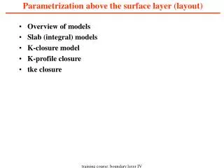
Parametrization above the surface layer (layout) • Overview of models • Slab (integral) models • K-closure model • K-profile closure • tke closure training course: boundary layer IV
Parametrization above the surface layer (layout) • Overview of models • Slab (integral) models • K-closure model • K-profile closure • tke closure training course: boundary layer IV
Parametrization above the surface layer (overview) training course: boundary layer IV
Parametrization above the surface layer (layout) • Overview of models • Slab (integral) models • K-closure model • K-profile closure • tke closure training course: boundary layer IV
Integral models • Integral models can be formally obtained by: • Making similarity assumption about shape of profile, e.g. • Integrate equations from • Solve rate equations for scaling parameters Mixed layer model of the day-time boundary layer is a well-known example of integral model. training course: boundary layer IV
Mixed layer (slab) model of day time BL This set of equations is not closed. A closure assumption is needed for entrainment velocity or for entrainment flux. training course: boundary layer IV
Closure for mixed layer model Buoyancy flux in inversion scales with production in mixed layer: CEis entrainment constant(0.2) Csrepresents shear effects (2.5-5) but is often not considered Closure is based on kinetic energy budget of the mixed layer: training course: boundary layer IV
Parametrization above the surface layer (layout) • Overview of models • Slab (integral) models • K-closure model • K-profile closure • tke closure training course: boundary layer IV
Grid point models with K-closure Levels in ECMWF model 91-level model 31-level model K-diffusion in analogy with molecular diffusion, but Diffusion coefficients need to be specified as a function of flow characteristics (e.g. shear, stability,length scales). training course: boundary layer IV
Diffusion coefficients according to MO-similarity Use relation between and to solve for training course: boundary layer IV
Louis formulation The Louis formulation specifies empirical functions of the Ri-number, whereas the MO-formulation specifies empirical functions of z/L. The two formulations are compatible in principle because: is equivalent to with training course: boundary layer IV
Stability functions FM,H based on Louis are very different from observational based (MO) (universal) functions. Louis’ functions provided larger exchanges for stable layers stable unstable training course: boundary layer IV
Geostrophic drag law Geostrophic drag law derived from single column simulations. Observations are from Wangara experiment. More drag MO-based FM,H give more realistic drag law, with less friction (A) and a larger ageostrophic angle (B) Larger ageos. angle training course: boundary layer IV
Single column simulations of stable BL • Three different forms of stability functions: • Derived from Monin Obukhov functions (based on observations) • Louis-Tiedtke-Geleyn (empirical Ri-functions) • Revised LTG with more diffusion for heat and less for momentum. Fm LTG Revised LTG MO Fh Revised LTG MO LTG training course: boundary layer IV
Stable BL diffusion Revised LTG has been designed to have more diffusion for heat, without changing the momentum budget Near surface cooling is sensitive to strength of FH training course: boundary layer IV
Stable BL diffusion Relaxation integration Jan 96; 2m T-diff.: Revised LTG - control training course: boundary layer IV
K-closure with local stability dependence (summary) • Scheme is simple and easy to implement. • Fully consistent with local scaling for stable boundary layer. • Realistic mixed layers are simulated (i.e. K is large enough to create a well mixed layer). • A sufficient number of levels is needed to resolve the BL i.e. to locate inversion. • Entrainment at the top of the boundary layer is not represented (only encroachment)! flux training course: boundary layer IV
Parametrization above the surface layer (layout) • Overview of models • Slab (integral) models • K-closure model • K-profile closure • tke closure training course: boundary layer IV
K-profile closure Troen and Mahrt (1986) Profile of diffusion coefficients: Find inversion by parcel lifting with T-excess: such that: See also Vogelezang and Holtslag (1996, BLM, 81, 245-269) for the BL-height formulation. h Heat flux training course: boundary layer IV
K-profile closure (ECMWF implementation) • Inversion interaction was too aggressive in original scheme and too much dependent on vertical resolution. • Features of ECMWF implementation: • No counter gradient terms. • Not used for stable boundary layer. • Lifting from minimum virtual T. • Different constants. • Implicit entrainment formulation. Entrainment fluxes zi Moisture flux Heat flux ECMWF entrainment formulation: ECMWF Troen/Mahrt C1 0.6 0.6 D 2.0 6.5 CE 0.2 - training course: boundary layer IV
Mixed layer parametrization Diffusion coefficients 1 2 0 Km/(kzu*) Mixed layer after 9 hours of heating from the surface by 100 W/m2 with 3 different parametrizations. Profiles of: Heat flux Potential temperature training course: boundary layer IV
Mixed layer parametrization Day time evolution of BL height from short range forecasts (composite of 9 dry days in August 1987 during FIFE) training course: boundary layer IV
Mixed layer parametrization Day time evolution of BL moisture from short range forecasts (composite of 9 dry days in August 1987 during FIFE) Louis-scheme K-profile OBS training course: boundary layer IV
Diurnal cycle over land Combination of drying from entrainment and surface moistening gives a very small diurnal cycle for q training course: boundary layer IV
K-profile closure (summary) • Scheme is simple and easy to implement. • Numerically robust. • Scheme simulates realistic mixed layers. • Counter-gradient effects can be included (might create numerical problems). • Entrainment can be controlled rather easily. • A sufficient number of levels is needed to resolve BL e.g. to locate inversion. training course: boundary layer IV
Parametrization above the surface layer (layout) • Overview of models • Slab (integral) models • K-closure model • K-profile closure • tke closure training course: boundary layer IV
TKE closure Eddy diffusivity approach: With diffusion coefficients related to kinetic energy: training course: boundary layer IV
Closure of TKE equation with closure: Main problem is specification of length scales, which are usually a blend of , an asymptotic length scale and a stability related length scale in stable situations. TKE from prognostic equation: training course: boundary layer IV
TKE (summary) Best to implement TKE on half levels. • TKE has natural way of representing entrainment. • TKE needs more resolution than first order schemes. • TKE does not necessarily reproduce MO-similarity. • Stable boundary layer may be a problem. training course: boundary layer IV