Chapter 9: Perfect Competition
Dive into the world of perfect competition economics, covering characteristics, profit maximization, supply and equilibrium, costs, and more. Learn how firms optimize decisions and maximize profit in a competitive market setting.

Chapter 9: Perfect Competition
E N D
Presentation Transcript
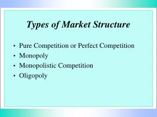
Chapter 9: Perfect Competition • Thus far we have examined how the consumer and firm attempt to optimize their decisions • The results of this optimization depend on the set-up of the economy • In this course we will examine the extreme set-ups: Perfect Competition and Monopoly
Chapter 9: Perfect Competition In this chapter we will cover: 9.1 Perfect Competition Characteristics 9.2 Economic and Accounting Profit 9.3 PC Profit Maximization 9.4 PC Short Run Supply and Equilibrium 9.5 PC Long Run Supply and Equilibrium 9.6 PC Costs 9.7 Economic Rent 9.8 Producer Surplus
9.1 Perfect Competition Characteristics • Fragmented Industry -Many buyers and sellers -No one buyer or seller has an effect on the industry -Each firm and consumer is a price taker (uses market price) 2) Homogeneous products -All firms produce identical products -No quality differences, no brand loyalty
Perfect Competition Characteristics 3) Perfect Information -Buyers and sellers have full information, especially regarding prices 4) No barriers to entry or exit -No input is restricted to potential customers or firms -Any firm or customer can enter or exit the market in the long run
Perfect Competition Characteristics As a result, we have: • Many buyers and sellers • Buying and selling identical goods At a given, set price. Note: although we are examining a market for outputs (goods and services), a similar analysis can apply to the market for inputs
9.2 Economic and Accounting Profit As seen before, Accounting Costs = Explicit Costs Economic Costs = Explicit Costs + Implicit Costs Furthermore, Accounting Profit = Revenue – Explicit Costs Economic Profit = Revenue – Explicit Costs - Implicit Costs
7.1.1 Implicit and Explicit Costs Explicit Costs: Costs that involve an exchange of money -ie: Rent, Wages, Licence, Materials Implicit Costs = Opportunity Costs: Costs that don’t involve an exchange of money; Cost of giving up the next best opportunity -ie: Wage that could have been earned working elsewhere; profitability of a goat if used mowing lawns instead of for meat
7.1.3 Economic and Accounting Costs Economists are interested in studying how firms make production & pricing decisions. They include all costs. Economic Costs = Explicit + Implicit Costs Accountants are responsible for keeping track of the money that flows into and out of firms. They focus on explicit costs. Accounting Costs = Explicit Costs Note: Different textbooks define costs differently. Refer to these notes for our class’ definitions.
Economic and Accounting Profit Implicit Costs are the BEST ALTERNATIVE return of ALL of an agent’s input (time, money, etc). Alternately, an agent’s time could earn a wage elsewhere. (ie: Work at Simtech for $3000 a month) An agent’s money both isn’t used currently and can be used elsewhere. (ie: Investing $5,000 @ 10% instead of using it to start a business gives an implicit cost of $500)
Economic Profit Accounting Profit Implicit Costs Revenue Revenue Economic Costs Explicit Costs Explicit Costs Profit: Economists vs Accountants Economist’s View Accountant’s View
7.1.2 Opportunity Cost Example Buck opens his own Bait shop in a store he owns, which cost $5,000 per month to run, but he makes $10,000 a month. Buck could have worked for Worms R Us for $2,000 per month, or rented out the store for $1,500 per month. Explicit Costs = $5,000 Accounting Profit = Revenue – Explicit Costs Accounting Profit = $10,000 - $5,000 Accounting Profit = $5,000
7.1.2 Opportunity Cost Example Buck opens his own Bait shop in a store he owns, which cost $5,000 per month to run, but he makes $10,000 a month. Buck could have worked for Worms R Us for $2,000 per month, or rented out the store for $1,500 per month. Implicit Costs = $2,000 (labour) + $1,500 (capital)Implicit Costs = $3,500 Econ Profit = Revenue – Explicit Costs – Implicit Costs Econ Profit = $10,000 - $5,000 - $3,500 Econ Profit = $1,500
Defining Sunk Cost Sunk Costs are costs that must be incurred no matter what the decision. These costs are not considered when making a future decision. Example: Talus Dome The Talus Dome was built in 2011 for $600,000. That cost is now SUNK, and shouldn’t be considered in any further analysis. (ie: Keep cleaning it or get rid of it) Picture Source: City of Edmonton Webpage (www.edmonton.ca)Price Source: Edmonton Journal
9.3 Profit Maximizing While previously we studied cost minimizing, in reality a firm is more concerned with maximizing its profits. Total Revenue: TR(Q)=PQ Total Cost: TC(Q) as found in previous chapters ie: TC(Q)=100+2Q Profit =Total Revenue – Total Cost: π(Q)=TR(Q)-TC(Q)
Review: TC(Q) TC(Q) in general is derived as follows: Originally: TC=wL+rK (1) Tangency Condition: L=f(K) (2) Production Function: Q=f(L,K) (3) (2) + (3) Q=f(L) and L=f(Q) (4) (2) + (4) K=f(Q) (5) (1) + (4) + (5) TC=wf(Q)+rf(Q) TC=f(Q)
Review: TC(Q) For Example: Originally: TC=wL+rK (1) Tangency Condition: L=K (2) Production Function: Q=2(LK)1/2 (3) (2) + (3) Q=2L and L=Q/2 (4) (2) + (4) K=Q/2 (5) (1) + (4) + (5) TC=wQ/2+rQ/2 TC=(w+r)Q/2
Marginal Revenue Definition: Marginal revenue is the change in revenue when output changes Marginal revenue is the slope of the total revenue curve. Since the PC firm is a price taker, the additional revenue gained from 1 additional output is EQUAL TO PRICE.
Marginal Revenue & Marginal Cost As seen previously, marginal cost changes as production increases. If for the next unit, MR>MC, that unit should be produced, as it yields profit. If for the last unit, MC>MR, that unit should not have been produced, as it decreases profit. Therefore profit is maximized where MC=MR=P
Total Cost, Total Revenue, Total Profit ($/yr) Total revenue = pq Total Cost Example: Profit Maximization Condition Total profit 15 q (units per year) MC P, MR 15 q (units per year) 6 30
The previous curves are expressed by: TC(q) = 242q - .9q2 + (.05/3)q3 MC(q) = 242 - 1.8q + .05q2 P = 15 At profit maximizing point: 1) P = MC But this occurs twice. At one point, profit is maximized, at another minimized. Therefore, in order to MAXIMIZE profit: 2) MC must be rising
Example In the paper industry, MC=20+2Q (which is always rising), where Q=100 reams of paper. Find the cost-maximizing quantity if P=30 or P=40 Solution: P=MC 30=20+2Q 5=Q P=MC 40=20+2Q 10=Q
Short Run Equilibrium In the short run, the firm either produces or temporarily shuts down, thus facing costs: STC(Q) = SFC + NSFC + TVC(q) when q > 0 = SFC when q = 0 SFC: Sunk Fixed costs – unavoidable sunk costs NSFC: Non-sunk Fixed costs – fixed costs that are avoidable if the firm temporarily shuts down TVC: Total Variable Costs; depends on output
9.4 Short Run Supply Definition: The firm’s Short run supply curve tells us how the profit maximizing output changes as the market price changes. HOWEVER, if the market price is too low, the firm will not operate in the short run. Ps = Shut down price (minimum market price where a firm will still operate)
9.4 Short Run Supply A firm will only operate if it can cover its NON SUNK COSTS. -ie: A sandwich shop will only stay open if it can pay its employees cover daily operating costs. 3 Cases: Case 1: all fixed costs are sunk Case 2: all fixed costs are non-sunk Case 3: some fixed costs are sunk
Case 1: Shut down price where SMC=AVC (all fixed costs are sunk – worst situation) $/yr SMC SAC AVC Ps Quantity (units/yr)
This firm may operate at a loss if P<SAC (Because operating has less loss than shutting down) $/yr SMC SAC AVC Ps Quantity (units/yr)
Case 2: Shut down Price where SMC=SAC (all costs are non-sunk – best case scenario) (This firm will never operate at a loss) $/yr SMC SAC Ps AVC Quantity (units/yr)
$/yr Case 3: Shut down price between SAC and AVC (sometimes called ANSC – Average non-sunk cost) (This firm operates at a loss if P<SAC) SMC SAC ANSC AVC Ps Quantity (units/yr)
At prices below SAC but above AVC, profits are negative if the firm produces…but the firm loses less by producing than by shutting down because of sunk costs. Example: STC(q) = 100 + 20q + q2 SFC = 100 (nb: this is sunk) TVC(q) = 20q + q2 AVC(q) = 20 + q SMC(q) = 20 + 2q
Calculate The Firm’s Supply Curve, • P = SMC • P = 20+2q • qs = ½P - 10 • If Market Price=$25, calculate firm production • qs = ½P - 10 • qs = ½(25) – 10 • qs = 2.5
If Market Price=$25, calculate firm profit/losses • qs = 2.5 • π=TR-TC • π=Pq-(100 + 20q + q2) • π=($25)2.5-(100 + 20(2.5) + (2.5)2) • π=62.5-(100 + 50 + 6.25) • π=-$93.75 • (remember that shutting down would have fixed costs of $100.)
P SMC SAC AVC Loss = $93.75 P* = $25 Ps = $20 Q q* = 2.5
Shut Down Rule Summary A firm will produce If It can cover its Non-Sunk Costs
Short Run Market Supply Curve and Short Run Market Equilibrium Thus far we have seen that the individual firm’s short run supply curve comes from their marginal cost curve. Definition: The market supply at any price is the sum of the quantities each firm supplies at that price. The short run market supply curve is the HORIZONTAL sum of the individual firm supply curves. (Just as market demand is the HORIZONTAL sum of individual demand curves)
Example: From Short Run Firm Supply Curve to Short Run Market Supply Curve Typical firm:Market: Individual supply curves per firm. 1000 firms of each type SMC3 $/unit SMC2 $/unit SMC1 Market supply 30 24 22 20 0 1.2 mill 0 300 400 500 q (units/yr) Q (m units/yr)
Short Run Perfectly Competitive Equilibrium Definition: A short run perfectly competitive equilibrium occurs when the market quantity demanded equals the market quantity supplied. ni=1 qs(P) = Qd(P) Qs(P)= Qd(P) and qs(P) is determined by the firm's individual profit maximization condition.
Example: Short Run Perfectly Competitive Equilibrium Typical firm:Market: $/unit $/unit Supply SMC SAC P* AVC Demand Ps q* Units/yr Q* m. units/yr
Example: Deriving a Short Run Market Equilibrium 300 identical firms Qd(P) = 60 – P STC(q) = 0.1 + 150q2 SMC(q) = 300q NSFC = 0 AVC(q) = 150q
a. Short Run Equilibrium Individual Firm: P = SMC P = 300q qs= P/300 Industry: Qs = 300(qs) Qs = P (for industry)
a. Short Run Equilibrium Market Price: Qs(P) = Qd(P) P = 60 – PP*= 30 Quantities: q* = P/300= 30/300q* = 0.1 Q* = PQ* = 30
b.Do firms make positive profits at the market equilibrium? SAC = STC/q SAC = 0.1/q + 150q SAC = 0.1/0.1 + 150(0.1) SAC = 16 Therefore, P* > SAC so profits are positive.
Comparative Statics in theShort Run • As seen in previous chapters, the entry or exit of firms or consumers, among other things, can shift the market demand and supply curves • Shifts in the market demand and supply curves will shift the equilibrium quantity as seen in chapters 1 and 2
The Long Run In the short run, capital is fixed and firms may temporarily operate under an economic profit or loss. In the long run, capital can change and firms can enter and leave the market, resulting in zero economic profit. Remember that in the long run, all costs are nonsunk (they are all avoidable at zero output)
Long Run MC Just as in the short run the firm operated at: P=SMC In the long run the firm operates at P=MC SMC≠MC (in general) since costs are reduced in the long run. Only at LR profit maximization is SMC=MC (because the short run is operating at the LR optimal capital point: Point A next slide)
In the long run, this firm has an incentive to change plant size to level K1 from K0: $/unit MC AC A SMC0 • SAC0 P SAC1 SMC1 q (000 units/yr) 1.8 6
9.5 LR Supply Curve In the long run, a firms supply curve is The firm’s LR MC curve above AC. For if P>AC, Profits>0. Since Profits = (PxQ)-(ACxQ) As in the short run, market supply is the horizontal sum of individual firm supply.
Long Run Supply Curve: $/unit MC S AC P SMC1 q (000 units/yr) 1.8 6
LR PC Equilibrium Long Run Perfectly Competitive Equilibrium occurs when: • Each firm maximizes profit with regards to output and capital (P=MC) • Each firm’s economic profit is zero (as firms keep entering until the price is pushed down to zero profits) (P=AC) • Market Demand=Market Supply
Long Run Perfectly Competitive Equilibrium Typical FirmMarket $/unit $/unit MC Market demand SAC AC P* SMC q*=50,000 Q*=10M. q Q
9.6 Long Run Costs • to increase production, a firm must increase inputs • Increasing MARKET output could change costs, therefore changing equilibrium price • A CONSTANT COST INDUSTRY is an industry where changes in output do not affect the price of inputs