Chapter 11: Monopoly

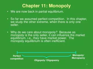
1. Monopoly/ Monopsony Perfect competition Oligopoly/ Oligopsony Chapter 11: Monopoly • We are now back in partial equilibrium. • So far we assumed perfect competition. In this chapter, we study the other extreme, when there is only one seller. • Why do we care about monopoly? Because as monopoly is the only seller, it can influence the market equilibrium, i.e., they have market power. The monopoly equilibrium is often inefficient.

2. Monopoly Profit Maximization • Being the only seller, monopoly can set price or quantity to influence the market equilibrium. • We know that all firms maximize their profits by setting MR=MC (as π=R-C). • Monopoly’s MC curve can be obtained in the same way as the competitive firms. • Difference is that monopoly faces a downward-sloping demand curve, thus it faces a different MR curve.

3. Marginal Revenue • Marginal revenue is the revenue the firm obtains from one more additional q.The MR is p for a competitive firm. • For monopoly: Thus, MR>0 if demand is elastic (ε<-1) MR<0 if demand is inelastic (-1<ε≤0). • If demand is inelastic, MR=MC is not optimum for a monopolist since MR<0. Come back to this point later.

4. MR= B = P*△Q =P B = P*△Q C = Q*△P MR = B +(-C)

5. Price 4 3 2 1 Example: Q = 4P -1 1 2 3 4 Quantity Unit Elastic Demand: What is MR?

6. Linear Demand Curve and MR For linear demand functions: p = a – bq, where a>0, b>0. R = pq = aq – bq2 MR= a – 2bq. • Thus, MR curve and demand curve have the same intercept, but MR is twice as steep as demand curve. • Elasticity at the mid-point is unity. • The demand is elastic when price is higher and inelastic when price is lower.

7. Elasticity of a Linear Demand Curve Price a ε< -1: elastic Demand: P = a - bq ε= -1 a/2 -1 < ε≤ 0: inelastic Marginal Revenue: P = a - 2bq a/b Quantity a/2b

8. Monopoly profit is maximized in the elastic portion of the demand. • A monopoly never operates in the inelastic portion of the demand. • A monopoly shuts down: • in LR if Pm<AC • In SR if Pm<AVC

9. Effects of a Shift of the Demand Curve • Unlike a competitive firm, a monopoly does not have a supply curve. Monopoly’s MC is not enough to know how much a monopoly will sell at any given price.

10. Market Power • Market power: the ability of a firm to charge P above MC and earn a positive profit. Q: Can a monopoly always set a very high price? • At profit-maximizing optimum: i.e., The ratio of P to MC depends only on the elasticity of demand at the optimum.

11. Lerner Index: the ratio of the difference between P and MC to the P (0≤LI ≤1). • The larger the LI, the greater the difference between p and MC, and thus the greater the monopoly’s market power. • LI=0 for competitive firm as it faces a perfectly elastic demand curve (ɛ=-∞).

12. Welfare Effects of Monopoly • Ch.9 showed that competitive equilibrium maximizes social welfare. • By setting higher price than MC, monopoly causes consumers to buy less than competitive equilibrium, which creates deadweight loss (DWL). • Thus, monopoly creates inefficiency.

13. Deadweight Loss of Monopoly

14. Since MC<Pm*, if the transaction of extra output (from Qm* to Qc*) takes place at MC<P<Pm*, both consumers and producer can be made better-off theoretically. • This is a Pareto improvement. • Why doesn’t monopolist do this, i.e. set different prices for the sale of extra output? • Monopolist cannot set different price levels for different consumers since resale is possible (but we study exceptions in the next chapter).

15. Imposing a tax on q

16. Imposing Ad Valorem (Sales) tax Because of the sales tax, the demand curve tilt

17. Effect of Ad Valorem Tax (1) Price MC pmb e* before tax e* for competitive market Demand MR qmb Quantity

18. Effect of Ad Valorem Tax (2) Price e* after tax MC pma_consumer pmb D MR （1-τ) MR qma Quantity （1-τ)D

19. Effects of Taxes on Welfare • Specific tax of t per q on monopolist: • Ad valorem tax of (τ×100)%: • Profit tax of (x×100)%

20. What Create Monopolies? Why does monopoly exist? • Natural monopoly: Small market demand relative to minimum efficient scale. One firm can produce the total output of the market at lower cost than several firms could. With a natural monopoly, it is more efficient to have only one firm produce than more firms. • Barriers to enter: Government grants monopoly rights to operate through licenses and restrictions. • Patent protection: Government provides monopoly right to use new idea for a certain period, to provide incentives to innovate.

21. Demand Relative to Minimum Efficient Scale (MES) Price Price Panel A: typical one firm’s AC curve If one firm produce Q*, the cost is too high. Panel B: there is a firm with Superior technology (ACs) ACs AC P* P* Demand Demand Q* Q* MES Output MES Output

22. Cost Advantages that Create Monopolies • Scale economies: Where MC curve =market demand curve, AC of a firm is still decreasing (see natural monopoly). • Scale economies can rise when production function is subject to increasing returns to scale. • Scale advantage can rise when fixed cost is large and MC is small. • Examples are electricity, gas, telephone, and so on requiring a lot of fixed costs. Other cases include superior technology (e.g., patent) and management ability.

23. A Natural Monopoly Price MC AC Demand PM PAC Loss to the firm from marginal cost pricing (p=MC) PMC MR qM qAC qMC Quantity

24. Dilemma is if p=MC by policy, profit is negative (purple area). • Solution I: Set p=MC and provide subsidy by the same amount as the deficit. • Solution II: Let public corporations supply. • “Solution” III: Permit the company which is willing to set the lowest price. This should be close to PAC.