Motion Control (wheeled robots)
890 likes | 1.81k Vues
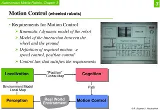
3. "Position". Localization. Cognition. Global Map. Environment Model. Path. Local Map. Real World. Perception. Motion Control. Environment. Motion Control (wheeled robots). Requirements for Motion Control Kinematic / dynamic model of the robot

Motion Control (wheeled robots)
E N D
Presentation Transcript
3 "Position" Localization Cognition Global Map Environment Model Path Local Map RealWorld Perception Motion Control Environment Motion Control (wheeled robots) • Requirements for Motion Control • Kinematic / dynamic model of the robot • Model of the interaction between the wheel and the ground • Definition of required motion -> speed control, position control • Control law that satisfies the requirements
3 Introduction: Mobile Robot Kinematics • Aim • Description of mechanical behavior of the robot for design and control • Similar to robot manipulator kinematics • However, mobile robots can move unbound with respect to its environment • there is no direct way to measure the robot’s position • Position must be integrated over time • Leads to inaccuracies of the position (motion) estimate -> the number 1 challenge in mobile robotics • Understanding mobile robot motion starts with understanding wheel constraints placed on the robots mobility
3.2.1 Introduction: Kinematics Model • Goal: • establish the robot speed as a function of the wheel speeds , steering angles , steering speeds and the geometric parameters of the robot (configuration coordinates). • forward kinematics • Inverse kinematics • why not -> not straight forward
3.2.1 Representing Robot Position • Representing to robot within an arbitrary initial frame • Initial frame: • Robot frame: • Robot position: • Mapping between the two frames • Example: Robot aligned with YI
3.2.1 Example
3.2.2 Forward Kinematic Models • Presented on blackboard
3.2.3 Wheel Kinematic Constraints: Assumptions • Movement on a horizontal plane • Point contact of the wheels • Wheels not deformable • Pure rolling • v = 0 at contact point • No slipping, skidding or sliding • No friction for rotation around contact point • Steering axes orthogonal to the surface • Wheels connected by rigid frame (chassis)
3.2.3 Wheel Kinematic Constraints:Fixed Standard Wheel
3.2.3 Example • Suppose that the wheel A is in position such that • a = 0 and b = 0 • This would place the contact point of the wheel on XI with the plane of the wheel oriented parallel to YI. If q = 0, then ths sliding constraint reduces to:
3.2.3 Wheel Kinematic Constraints:Steered Standard Wheel
3.2.3 Wheel Kinematic Constraints:Castor Wheel
3.2.3 Wheel Kinematic Constraints:Swedish Wheel
3.2.3 Wheel Kinematic Constraints:Spherical Wheel
3.2.4 Robot Kinematic Constraints • Given a robot with M wheels • each wheel imposes zero or more constraints on the robot motion • only fixed and steerable standard wheels impose constraints • What is the maneuverability of a robot considering a combination of different wheels? • Suppose we have a total of N=Nf + Ns standard wheels • We can develop the equations for the constraints in matrix forms: • Rolling • Lateral movement
3.2.5 Example: Differential Drive Robot • Presented on blackboard
3.2.5 Example: Omnidirectional Robot • Presented on blackboard
3.3 Mobile Robot Maneuverability • The maneuverability of a mobile robot is the combination • of the mobility available based on the sliding constraints • plus additional freedom contributed by the steering • Three wheels is sufficient for static stability • additional wheels need to be synchronized • this is also the case for some arrangements with three wheels • It can be derived using the equation seen before • Degree of mobility • Degree of steerability • Robots maneuverability
3.3.1 Mobile Robot Maneuverability: Degree of Mobility • To avoid any lateral slip the motion vector has to satisfy the following constraints: • Mathematically: • must belong to the null space of the projection matrix • Null space of is the space N such that for any vector n in N • Geometrically this can be shown by the Instantaneous Center of Rotation (ICR)
3.3.1 Mobile Robot Maneuverability: Instantaneous Center of Rotation • Ackermann Steering Bicycle
3.3.1 Mobile Robot Maneuverability: More on Degree of Mobility • Robot chassis kinematics is a function of the set of independent constraints • the greater the rank of , the more constrained is the mobility • Mathematically • no standard wheels • all direction constrained • Examples: • Unicycle: One single fixed standard wheel • Differential drive: Two fixed standard wheels • wheels on same axle • wheels on different axle
3.3.2 Mobile Robot Maneuverability: Degree of Steerability • Indirect degree of motion • The particular orientation at any instant imposes a kinematic constraint • However, the ability to change that orientation can lead additional degree of maneuverability • Range of : • Examples: • one steered wheel: Tricycle • two steered wheels: No fixed standard wheel • car (Ackermann steering): Nf = 2, Ns=2 -> common axle
3.3.3 Mobile Robot Maneuverability: Robot Maneuverability • Degree of Maneuverability • Two robots with same are not necessary equal • Example: Differential drive and Tricycle (next slide) • For any robot with the ICR is always constrained to lie on a line • For any robot with the ICR is not constrained an can be set to any point on the plane • The Synchro Drive example:
3.3.3 Mobile Robot Maneuverability: Wheel Configurations • Differential Drive Tricycle
3.3.3 Five Basic Types ofThree-Wheel Configurations
3.3.3 Synchro Drive
3.4.1 Mobile Robot Workspace: Degrees of Freedom • Maneuverability is equivalent to the vehicle’s degree of freedom (DOF) • But what is the degree of vehicle’s freedom in its environment? • Car example • Workspace • how the vehicle is able to move between different configuration in its workspace? • The robot’s independently achievable velocities • = differentiable degrees of freedom (DDOF) = • Bicycle: DDOF = 1; DOF=3 • Omni Drive: DDOF=3; DOF=3
3.4.2 Mobile Robot Workspace: Degrees of Freedom, Holonomy • DOF degrees of freedom: • Robots ability to achieve various poses • DDOF differentiable degrees of freedom: • Robots ability to achieve various path • Holonomic Robots • A holonomic kinematic constraint can be expressed a an explicit function of position variables only • A non-holonomic constraint requires a different relationship, such as the derivative of a position variable • Fixed and steered standard wheels impose non-holonomic constraints
3.4.2 Mobile Robot Workspace:Examples of Holonomic Robots
3.4.3 Path / Trajectory Considerations: Omnidirectional Drive
3.4.3 Path / Trajectory Considerations: Two-Steer
3.5 Beyond Basic Kinematics
3.6 Motion Control (kinematic control) • The objective of a kinematic controller is to follow a trajectory described by its position and/or velocity profiles as function of time. • Motion control is not straight forward because mobile robots are non-holonomic systems. • However, it has been studied by various research groups and some adequate solutions for (kinematic) motion control of a mobile robot system are available. • Most controllers are not considering the dynamics of the system
3.6.1 Motion Control: Open Loop Control • trajectory (path) divided in motion segments of clearly defined shape: • straight lines and segments of a circle. • control problem: • pre-compute a smooth trajectory based on line and circle segments • Disadvantages: • It is not at all an easy task to pre-compute a feasible trajectory • limitations and constraints of the robots velocities and accelerations • does not adapt or correct the trajectory if dynamical changes of the environment occur. • The resulting trajectories are usually not smooth
3.6.2 Motion Control: Feedback Control,Problem Statement • Find a control matrix K, if exists with kij=k(t,e) • such that the control of v(t) and w(t) • drives the error e to zero.
3.6.2 Dy Motion Control:Kinematic Position Control The kinematic of a differential drive mobile robot described in the initial frame {xI, yI, q} is given by, where and are the linear velocities in the direction of the xIand yI of the initial frame. Let a denote the angle between the xR axis of the robots reference frame and the vector connecting the center of the axle of the wheels with the final position.
3.6.2 Dy Kinematic Position Control: Coordinates Transformation Coordinates transformation into polar coordinates with its origin at goal position: System description, in the new polar coordinates for for
3.6.2 Kinematic Position Control: Remarks • The coordinates transformation is not defined at x = y = 0; as in such a point the determinant of the Jacobian matrix of the transformation is not defined, i.e. it is unbounded • For the forward direction of the robot points toward the goal, for it is the backward direction. • By properly defining the forward direction of the robot at its initial configuration, it is always possible to have at t=0. However this does not mean that a remains in I1 for all time t.
3.6.2 Kinematic Position Control: The Control Law • It can be shown, that withthe feedback controlled system • will drive the robot to • The control signal v has always constant sign, • the direction of movement is kept positive or negative during movement • parking maneuver is performed always in the most natural way and without ever inverting its motion.
3.6.2 Kinematic Position Control: Resulting Path
3.6.2 Kinematic Position Control: Stability Issue • It can further be shown, that the closed loop control system is locally exponentially stable if • Proof: for small x -> cosx = 1, sinx = xand the characteristic polynomial of the matrix A of all roots have negative real parts.
3.XX Mobile Robot Kinematics: Non-Holonomic Systems • Non-holonomic systems • differential equations are not integrable to the final position. • the measure of the traveled distance of each wheel is not sufficient to calculate the final position of the robot. One has also to know how this movement was executed as a function of time. s1=s2 ; s1R=s2R ; s1L=s2L but: x1 = x2 ; y1 = y2
3.XX Non-Holonomic Systems: Mathematical Interpretation • A mobile robot is running along a trajectory s(t). At every instant of the movement its velocity v(t) is: • Function v(t) is said to be integrable (holonomic) if there exists a trajectory function s(t) that can be described by the values x, y, and q only. • This is the case if • With s = s(x,y,q) we get for ds Condition for integrable function
3.XX Non-Holonomic Systems: The Mobile Robot Example • In the case of a mobile robot where • and by comparing the equation above with • we find • Condition for an integrable (holonomic) function: • the second (-sinq=0) and third (cosq=0) term in equation do not hold!