Motion Planning
Motion Planning. Howie CHoset. Why do we want robots?. Why do we want robots?. Dirty Dull Dangerous. Why do we want robots?. Dirty Dull Dangerous Delicate. Why do we want robots?. Dirty Dull Dangerous Delicate Expense. Why do we want robots?. Dirty Dull Dangerous Delicate

Motion Planning
E N D
Presentation Transcript
Motion Planning Howie CHoset
Why do we want robots? • Dirty • Dull • Dangerous
Why do we want robots? • Dirty • Dull • Dangerous • Delicate
Why do we want robots? • Dirty • Dull • Dangerous • Delicate • Expense
Why do we want robots? • Dirty • Dull • Dangerous • Delicate • Expense • Entertainment • Education
Motion Planning Howie CHoset
What is Motion Planning? • Determining where to go
Overview • The Basics • Motion Planning Statement • The World and Robot • Configuration Space • Metrics • Path Planning Algorithms • Start-Goal Methods • Map-Based Approaches • Cellular Decompositions • Applications • Navigating Large Spaces • Coverage
The World consists of... • Obstacles • Already occupied spaces of the world • In other words, robots can’t go there • Free Space • Unoccupied space within the world • Robots “might” be able to go here • To determine where a robot can go, we need to discuss what a Configuration Space is
Motion Planning Statement If W denotes the robot’s workspace, And Cidenotes the i’th obstacle, Then the robot’s free space, FS, is defined as: FS = W - ( U Ci ) And a path c C0is c : [0,1] g FS where c(0) is qstart and c(1) is qgoal
Free Space Obstacles Robot x,y Example of a World (and Robot)
Basics: Metrics • There are many different ways to measure a path: • Time • Distance traveled • Expense • Distance from obstacles • Etc…
Bug 1 • known direction to goal • otherwise local sensing • walls/obstacles & encoders But some computing power! “Bug 1” algorithm 1) head toward goal 2) if an obstacle is encountered, circumnavigate it and remember how close you get to the goal 3) return to that closest point (by wall-following) and continue Vladimir Lumelsky & Alexander Stepanov: Algorithmica 1987
Bug 1 • known direction to goal • otherwise local sensing • walls/obstacles & encoders But some computing power! “Bug 1” algorithm 1) head toward goal 2) if an obstacle is encountered, circumnavigate it and remember how close you get to the goal 3) return to that closest point (by wall-following) and continue Vladimir Lumelsky & Alexander Stepanov: Algorithmica 1987
Bug2 Call the line from the starting point to the goal the m-line “Bug 2” Algorithm
A better bug? Call the line from the starting point to the goal the m-line “Bug 2” Algorithm 1) head toward goal on the m-line
A better bug? Call the line from the starting point to the goal the m-line “Bug 2” Algorithm 1) head toward goal on the m-line 2) if an obstacle is in the way, follow it until you encounter the m-line again.
A better bug? “Bug 2” Algorithm m-line 1) head toward goal on the m-line 2) if an obstacle is in the way, follow it until you encounter the m-line again. 3) Leave the obstacle and continue toward the goal OK ?
A better bug? “Bug 2” Algorithm 1) head toward goal on the m-line 2) if an obstacle is in the way, follow it until you encounter the m-line again. 3) Leave the obstacle and continue toward the goal Start Goal Better or worse than Bug1?
A better bug? “Bug 2” Algorithm 1) head toward goal on the m-line 2) if an obstacle is in the way, follow it until you encounter the m-line again. 3) Leave the obstacle and continue toward the goal Start Goal NO! How do we fix this?
A better bug? “Bug 2” Algorithm 1) head toward goal on the m-line 2) if an obstacle is in the way, follow it until you encounter the m-line again closer to the goal. 3) Leave the obstacle and continue toward the goal Start Goal Better or worse than Bug1?
Lumelsky Bug Algorithms • Unknown obstacles, known start and goal. • Simple “bump” sensors, encoders. • Choose arbitrary direction to turn (left/right) to make all turns, called “local direction” • Motion is like an ant walking around: • In Bug 1 the robot goes all the way around each obstacle encountered, recording the point nearest the goal, then goes around again to leave the obstacle from that point • In Bug 2 the robot goes around each obstacle encountered until it can continue on its previous path toward the goal
Assumptions • Size of robot • Perfect sensing • Perfect control • Localization (heading) What else?
What is the position of the robot? Expand obstacle(s) Reduce robot not quite right ...
Free Space Obstacles Robot x,y Example of a World (and Robot)
Free Space Obstacles Robot (treat as point object) x,y Configuration Space: Accommodate Robot Size
Trace Boundary of Workspace Pick a reference point…
Translate-only, non-circularly symmetric Pick a reference point…
The Configuration Space • What it is • A set of “reachable” areas constructed from knowledge of both the robot and the world • How to create it • First abstract the robot as a point object. Then, enlarge the obstacles to account for the robot’s footprint and degrees of freedom • In our example, the robot was circular, so we simply enlarged our obstacles by the robot’s radius (note the curved vertices)
Attractive/Repulsive Potential Field • Uatt is the “attractive” potential --- move to the goal • Urep is the “repulsive” potential --- avoid obstacles
Artificial Potential Field Methods:Attractive Potential Quadratic Potential
The Wavefront Planner • A common algorithm used to determine the shortest paths between two points • In essence, a breadth first search of a graph • For simplification, we’ll present the world as a two-dimensional grid • Setup: • Label free space with 0 • Label start as START • Label the destination as 2
Representations • World Representation • You could always use a large region and distances • However, a grid can be used for simplicity
Representations: A Grid • Distance is reduced to discrete steps • For simplicity, we’ll assume distance is uniform • Direction is now limited from one adjacent cell to another • Time to revisit Connectivity (Remember Vision?)
Representations: Connectivity • 8-Point Connectivity • 4-Point Connectivity • (approximation of the L1 metric)
The Wavefront in Action (Part 1) • Starting with the goal, set all adjacent cells with “0” to the current cell + 1 • 4-Point Connectivity or 8-Point Connectivity? • Your Choice. We’ll use 8-Point Connectivity in our example
The Wavefront in Action (Part 2) • Now repeat with the modified cells • This will be repeated until no 0’s are adjacent to cells with values >= 2 • 0’s will only remain when regions are unreachable
The Wavefront in Action (Part 3) • Repeat again...