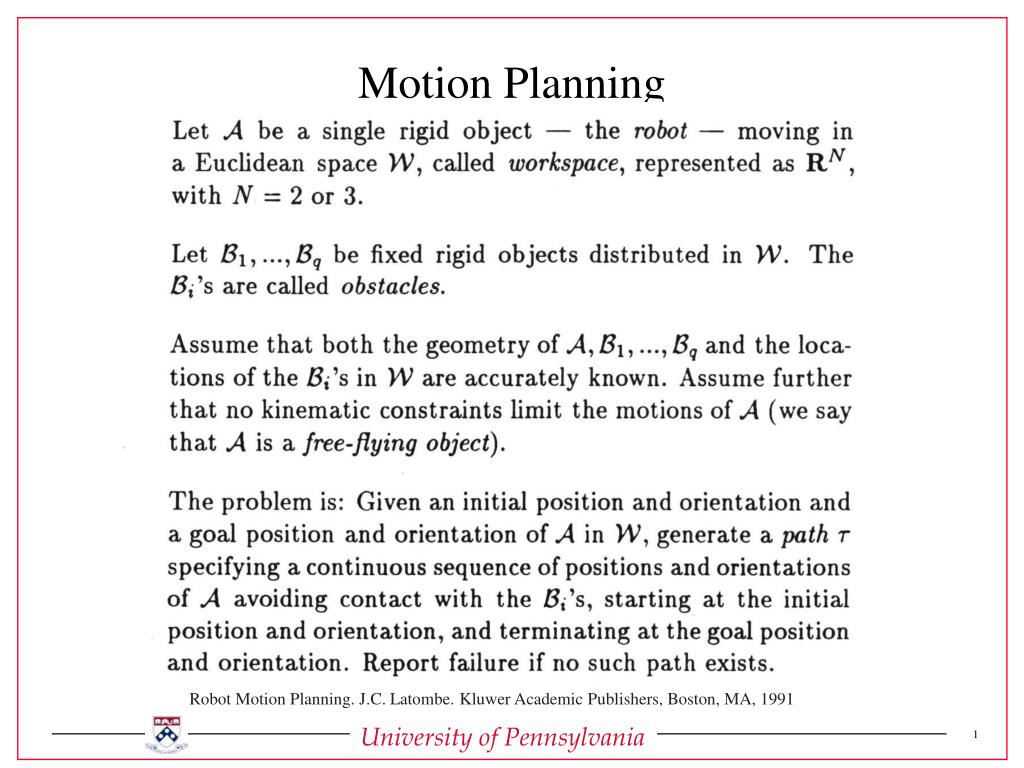
1. Motion Planning Robot Motion Planning. J.C. Latombe. Kluwer Academic Publishers, Boston, MA, 1991

2. Trajectory generation • Given end points (and possibly intermediate points) and velocities, generate a smooth trajectory between them while avoiding obstacles and obeying constraints

3. Explicit Motion Planning Motion Planner subgoals Trajectory Generator smooth trajectory Controller • Signals to joint controllers/drivers • joint velocities • joint torques

4. Control Find a control input u(t) Robot Motion Planning. J.C. Latombe. Kluwer Academic Publishers, Boston, MA, 1991

5. Known Environments (Model) Explicit motion plans Implicit motion plans Unknown Environments Sensor based motion planning Usually combines Motion Planning Trajectory Generation Control Motion Planning

6. Earliest Implicit Motion Planning Algorithm 1. The robot follows a straight line segment to the goal. 2. When it hits an obstacle (at the hitting point), it follows its boundary while keeping track of the straight line segment. 3. When it returns to the hitting point, it follows the boundary to the point on the boundary that is on the line segment and closest to the goal. 4. It then resumes the straight line segment path to the goal. Always finds a path (if it exists) Bug Algorithm: Vladimir Lumelsky

7. Implicit Method: Potential Field Controllers • Basic idea • Create attractive potential field to pull robot (R) toward a goal • Create repulsive potential field to repel robot (R) from obstacles • In two-dimensional space (robot is a point, goal/obstacles are points) • Remember: Force on a particle is given by f = -grad (V)

8. Implicit Method: Potential Field Controllers • Basic idea • Construct potential field for goal • Construct potential field for each obstacle • Add potential fields to create the total potential V(x, y) Assume two-dimensional space (robot is a point) • Force on a particle is given by f = -grad (V) • Command robot velocity according to the following control law (policy)

9. Basic idea Attractive potential field for goal Repulsive potential field for obstacles Attractive + repulsive potential fields Equi-potential contours Force field [Latombe 91]

10. Potential Field: Goal (x=0.5, y=0.5) Contour plot of Vgoal

11. Potential Field: Obstacle (x=0.0, y=0.0) Contour plot of Vobs

12. Vobs + 100 Vgoal

13. Trajectory for Vobs + 500 Vgoal

14. Application to Articulated Arms Eight-Jointed Planar Arm [Latombe 91]

15. What are the potential (no pun!) difficulties?

16. From Potential Functions to Navigation Functions • Consider sphere worlds • D.E. Koditschek and E. Rimon,”Robot Navigation Functions on Manifolds with boundary”, Advances in Applied Mathematics, vol. 11, pages 412-442, 1990 • E. Rimon and D.E. Koditschek, “Exact Robot Navigation Using Artificial Potential Functions”, IEEE Transactions on Robotics and Automation, vol. 8 (5), pages 501-518, 1992

17. Key Observation for Sphere Worlds • A globally attracting equilibrium state is not possible. • There must be at least as many saddle points as there are obstacles • Each obstacle introduces at least one saddle point

18. f is differentiable f has a unique minimum Critical points of f are isolated (i.e., non degenerate) Navigation Functions