Jet-jet angular distributions Blessing
800 likes | 819 Vues
Investigating quark substructure via angular distributions & MC simulation. Explore sensitivity & systematics in high-mass dijet data. Discover insights on jet energy scale & parton distribution functions.

Jet-jet angular distributions Blessing
E N D
Presentation Transcript
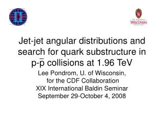
Jet-jet angular distributions Blessing Lee Pondrom and Yeongdae Shon University of Wisconsin September 18, 2008
Data Sample • 1.1 fb¹ integrated luminosity • 12 million jet100 triggers • 10 nb constant trigger cross section
Minimal cuts • ||<2 • |Zvertex|<60 cm • Missing ET significance < 5 GeV
QCD 22 angular distributions • The formulas of Combridge for q+qq+q, q+qbarq+qbar, q+qbarg+g, q+gq+g, g+gg+g, and g+gq+qbar give angular distributions which resemble Rutherford’s formula dd~1/sin4(*/2). Rutherford’s formula is flat in exp(|2|) Where ’s refer to the two leading jets
Jet-jet angular distribution and quark substructure • Quark substructure effective contact color singlet Lagrangian of Eichten, et al is: • L = ±(g²/2Λ²(LLLL • Looks just like muon decay. Affects only the quarks. Color singlet means that some diagrams have no interference term. Correct formulas with interference are in CDFR3637. • g²/4 = 1; strength of the interaction ~(ŝ/²)² _ _ _
Effect of quark substructure • The quark substructure Lagrangian is basically isotropic, so the angular distribution near *=, or is most sensitive to . • The ET distribution also depends on , but is more sensitive to the jet energy scale than the angular distribution in a given mass bin.
treatment of the data • Divide the data into four bins in jet-jet invariant mass, using the two highest ET jets in the event. Do not look for third jets. • Each bin is 100 GeV wide, starting at 550-650 GeV, and ending at 850-950 GeV.
Monte Carlo predicts the expected QCD distributions, and the effects of quark substructure • The MC program used is Pythia. • Pythia generates the QCD event at the ‘hadron level’, without the CDF detector simulation, via a multistep process involving ISR, 22,FSR, and parton fragmentation. • Hadron level events are then subject to the full CDF detector simulation, and analyzed with the same code as data.
Distribution sensitivity to • A ratio method was used to measure the effect of on the angular distribution in a given mass bin. • Define R=(1<<10)/(15<<25). • Using Pythia for the dependence, plot R()/R() versus (mass)4, where R() means no quark substructure.
To obtain a limit we must understand the systematics • Sensitivity to the choice of the parton distribution functions. We are looking at high mass dijets, searching for quark substructure, so the most important pdf’s are proton valence valence. • The first study compared CTEQ and MRST.
Systematics of the pdf’s • MRSTLO ‘high s’ and CTEQ5L predict the same angular distributions with no quark substructure. • There is a new method for evaluating uncertainties from the pdf’s, using ‘vectors’ which represent 1 variation coming from the input experimental data.
Systematic studies continued • Choice of Q2. Here the angular distributions differ. Vary the mix of ŝ and pT2 by 1. • The jet energy scale. Use the utility to vary the jet energy corrections by ±1. The high mass jet-jet cross section depends on the jet energy corrections.
Procedure • Calculate R for three MC samples: best fit, +1 and -1, varying the choice of Q2. • Do a simple average <R>=(R1+R2+R3)/3 • Calculate R for three data samples:level7 jetEcorrections, +1 and -1. • Again do a simple average <Rd>=(R1d+R2d+R3d)/3
Systematic uncertainties • The systematics are included in the uncertainty in each ratio by summing the deviations from the mean: dR² = i=1,3(Ri-<R>)²/2 for the MC, and similarly for dR²d. • Then the final ratios Rd/R are calculated for each mass bin, and plotted vs (mass)4
Summary • The ratio R=(110)/(1525) shows a linear dependence vs x=(mass)4 , with a slope which increases with increasing . • The data have a slope which is slightly negative: dR/dx = -0.160.08. This result is unphysical. • To set a limit, we use the Feldman Cousins method (PRD 57,3873 (1998)).
Feldman Cousins method • The method is based on physically allowed results versus experimental results, which can be unphysical. • The uncertainties must be known, but not the result. • For a set of allowed results, generate all possible outcomes, using the uncertainties.
Procedure • Eight input slopes were chosen, in steps of .05, between 0 and 0.4. • For each input slope, the output was obtained by Gaussian variation using the known uncertainties, including systematics • 20,000 ‘psuedo-experiments’ were performed for each input. • The resulting curves are normalized to one.
Feldman Cousins renormalization • The next step is to renormalize the curves, by finding the maximum in each vertical tower, giving a box in x and y. • Then each box in that y row is divided by the maximum. • This gives step 2.
Final limits • By integration, 95% and 68% confidence contours can be extracted from this plot.
Limits from the plot • From the intersection of the measured slope with the confidence level contours, we conclude: • Slope<0.24 95% confidence • Slope<0.06 68% confidence • Expected slope limit for zero slope result (based on these experimental uncertainties) slope<0.35
Conclusions • To interpret these slopes as lower limits on the quark substructure parameter , we must rely on Pythia Monte Carlo simulation, which gives the sensitivity of the slope of the angular distribution ratio to . • 95% confidence >2.4 TeV • 68% confidence >3.5 TeV • 95% confidence expected result >2.2 TeV
Requested material • Three topics are covered. Not part of the blessing. • 1. Extra jetEnergy uncertainty in the plug • 2. Hadron level corrections from Pythia • 3. Trigger threshold at 100 GeV in the Monte Carlo
Check of the effect of the extra plug uncertainties • The normal level7 jetEcorrections package was run on 5M data jet100 events • The supplied uncertainty formula was applied only to those jets (1.1<|det|<2.1) • Central jets were not affected.
Conclusion of the plug uncertainty exercise • Hardly any visible effect.
Hadron level correctionsnotice how flat the had level distributions are
Monte Carlo trigger • The conclusion here is that, while the distribution of the Monte Carlo in the 550-650 GeV mass bin does not exactly match the data, and the resulting 2 is bad, the discrepancy is not due to the trigger turn on. • There are small discrepancies in all of the plots, and each bin in has over 1000 events.
CTEQ6 and the vectors • Only CTEQ6 has the vectors. Earlier versions, like the default CTEQ5L used here, do not. • There are 40 vectors, in pairs up and down. They are linearly independent • It is not obvious which vectors affect specific pdf’s – like up quarks.
CTEQ6 and the vectors cont’d • Preliminary studies with the full Pythia Monte Carlo, but without the CDF detector simulation, show that the vector effect is small. • Conclusion: The lack of knowledge of the pdf’s is not an important contributor to the systematic uncertainty.
This is the analysis for which blessing is requested • The following slides were requested after the June 12 presentation. • Correction of the data to the hadron level is necessary to compare to NLOJet++, a subject which we prefer to postpone at the present time. The analysis for preblessing compares data as taken with fully simulated Monte Carlo.
Further studies with Nlojet++ • NLO QCD C++ code written by Zoltan Nagy (arXiv:hep-ph/0110315) • Downloadable from CERN • Born+nlo calculations with 5E9 events • Three partons in the final state, pairs clustered in cone 0.7 merged to one ‘jet’. • Hard scale 0=ETave and 0=mjj match Pythia choices
Data hadron level corrected compared to Pythia for Q2=pT2 +ŝ