Download
1 / 19
200 likes | 229 Vues
Creating bullet charts in Excel can be a bit tricky. This slidedeck lays out a step-by-step approach to creating bullet charts in Excel. The approach was first made public by Jorge Camoes (http://www.excelcharts.com/blog/easy-way-make-bullet-charts-boxplots-excel/). An alternative version was published in early 2011 by Jon Peltier (http://peltiertech.com/WordPress/how-to-make-horizontal-bullet-graphs-in-excel/). The Excel file is available on my website (http://policyviz.com/a-step-by-step-guide-to-making-bullet-charts-in-excel).

E N D
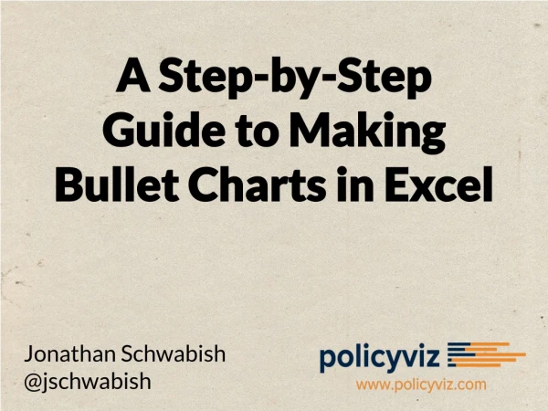
A Step-by-Step Guide to Making Bullet Charts in Excel Bullet Charts in Excel A Step-by-Step Guide to Making Jonathan Schwabish @jschwabish
Here is the bullet chart we will make. Bullet charts are made up of four main parts: 1. Background fill colors encode ranges (for example, low, medium, and high) 2. Label 3. Bar shows actual performance 4. Marker shows target performance
Step 1. The bullet chart is created from a scatterplot. To start, set up your data with one column that will serve as the y-axis values and separate columns for each of the series in the chart. Start with a connected scatterplot with the first series (Low).
Step 3. Here’s what you have after all 6 series have been added to the chart.
Step 4. Select the first series and change the ‘Marker Type’ to none.
Step 5. Go to the ‘Line Style’ menu. We will make two changes here. First, change the width to, say, 12 pt.
Step 6. Second, change the ‘Cap Type’ to ‘Flat’. It’s important to use Flat because this brings the line right to the data points.
Step 7. Notice that if you use the ‘Square’ option, the line overlaps the data points.
Step 8. Repeat the process for the other series. Make the ‘Actual’ series a slightly thinner width, say, 5 pt.
Step 9. You can change the Outline color on all the series to the colors you choose. (Note that because these are lines, you will use the Outline color, not the Fill color.)
Step 10. We’ll now make three changes to the label the chart (using the “Unit, 2012” series). First, add a data label; second, align it to the left; and third, set the marker to ‘None’.
Step 11. You can then modify the y-axis scale to center the chart in the graph space.
Step 12. You can also modify the x-axis scale for the same reason.
Step 13. Now delete the legend, axes, and gridlines. You are left with a nice, single bullet chart
You can add other bullet charts by adding more data and repeating the process. 1st series 2nd series
You can also change the shape of the Target level—say, to a vertical line—by drawing a line in your worksheet and then copying and pasting it directly onto the ‘Target’.
And now you have two bullet charts. Unit, 2013 Unit, 2012
Attributions The method presented here was first made public by Jorge Camoes. For an alternative approach, see Jon Peltier. Textured background from Chris Spooner. Excel file is available here. Jonathan Schwabish @jschwabish