Download
1 / 48
480 likes | 498 Vues
A detailed numerical formulation for the Horizontal Grid Hybrid 3 and Vertical Grid SZ, including the Terrain-following zone, CZ, and VQS. The method utilizes the Localized Sigma Coordinates and a semi-implicit scheme for continuity and momentum equations. It also incorporates a Galerkin finite-element formulation for the continuity and momentum equations. Additionally, an overview of the Galerkin weighted residual statement and shape function integration is provided.

E N D
Horizontal grid: hybrid 3 Side 2 4 3 Side 1 Side 2 Side 1 Side 3 Side 4 1 2 2 1 Side 3 3 2 1 1 2 3 3 2 ys 2 2 i Ni 1 xs 1 1 Ni i 2 1 i Ni Ni 1
Vertical grid: SZ Terrain-following zone z SZ zone s zone S zone s=0 Nz hc hs hs S-levels kz s=-1 kz-1 Z-levels 2 1
S-coordinates qf=10-3, any qb qf=10, qb=1 hc qf=10, qb=0 qf=10, qb=0.7
Vertical grid: SZ z=-hs
LSC2 via VQS Dukhovskoy et al. (2009)
A What to do with the staircases? u u P 1 2 B Q R 1 2 LSC2= Localized Sigma Coordinates with Shaved Cells (ivcor=1 in vgrid.in)
Vertical grid: LSC2 z (m) Degenerate prism
Vertical grid (3) • 3D computational unit: uneven prisms • Equations are not transformed into S- or s-coordinates, but solved in the original Z-space • PGE • Z-method with cubic spline (extrapolation on surface/bottom) nk nk k k(whole level) Nz h Nz-1 uj,k+1vj,k+1 h uj,k+1vj,k+1 ……. k Ci,k Ci,k k-1 k-1 ……. k-1 wi,k-1 kb+1 wi,k-1 kb
Polymorphism Bathymetry (m)
Polymorphism flood z (m) x (m) S (PSU)
Semi-implicit scheme Continuity • Implicit treatment of divergence and pressure gradient (and SAV) terms by-passes most severe stability constraints: 0.5 ≤q≤1 • Explicit treatment: Coriolis, baroclinicity, horizontal viscosity, radiation stress… Momentum b.c. Advection:
Characteristic line t+Dt t Eulerian-Lagrangian Method • ELM: takes advantage of both Lagrangian and Eulerian methods • Grid is fixed in time, and time step is not limited by Courant number condition • Advections are evaluated by following a particle that starts at certain point at time t and ends right at a pre-given point at time t+Dt. • The process of finding the starting point of the path (foot of characteristic line) is called backtracking, which is done by integrating dx/dt=u3 backward in 3D space and time. • To better capture the particle movement, the backward integration is often carried out in small sub-time steps • Simple backward Euler method • 2nd-order R-K method • Interpolation-ELM does not conserve; integration ELM does • Interpolation: numerical diffusion vs. dispersion advection dispersion diffusion Diffusion Dispersion CFL>0.4
Operating range of SCHISM …. for a fixed grid Convergence: CFL=const, Dt0
x ELM with high-order Kriging • Best linear unbiased estimator for a random function f(x) • “Exact” interpolator • Works well on unstructured grid (efficient) • Needs filter (ELAD) to reduce dispersion Cubic spline Drift function Fluctuation K is called generalized covariance function Minimizing the variance of the fluctuation we get 2-tier Kriging cloud • The numerical dispersion generated by kriging is reduced by a diffusion ELAD filter (Zhang et al. 2016)
Semi-implicit scheme Continuity • Implicit treatment of divergence and pressure gradient terms by-passes most severe CFL condition : 0.5 ≤q≤1 • Explicit treatment: Coriolis, baroclinicity, horizontal viscosity, radiation stress… Momentum b.c.
Galerkin finite-element formulation A Galerkin weighted residual statement for the continuity equation: Vertical integration of the momentum equation Shape function (1) 2D case:
ub db Galerkin finite-element formulation Vertical integration of the momentum equation (2) 3D case: z=-h Momentum equation applied to the bottom boundary layer via Vertically integrated velocity becomes (friction-modified depth) Write in a unified compact form Note the difference in between 2D/3D!
Finite-element formulation (cont’d) I1 Finally, substituting this eq. back to continuity eq. we get one equation for elevations alone: I3 I5 I4 I6 source (i=1,…,Np) • Notes: • When node i is on boundaries where essential b.c. is imposed, h is known and so no equations are needed, and so I2 and I6 need not be evaluated there • When node i is on boundaries where natural b.c. is imposed, the velocity is known and so the last term on LHS is known only the first term is truly unknown!
x j j-1 j+1 N 1 x j j-1 j+1 N 1 Shape function • Used to approximate the unknown function • Although usually used within each individual elements, shape function is global not local! • Must be sufficiently smooth to allow integration by part in weak formulation • Mapping between local and global coordinates • Assembly of global matrix Conformal Non-conformal (Elevation) (optional velocity)
Matrices: I1 i34(j) Wj i i’ is local index of node iin Wj. reaches its max when i’=l, and so does I1. i’ so diagonal is dominant if the averaged friction-reduced depth ≥0 (can be relaxed) Mass matrix is positive definite and symmetric! JCG solver > (i’,2) (i’,1)
Matrices: I3 and I5 n j i Gij j Flather b.c. (overbar denotes mean) Similarly
Matrices: I7 Related to source/sink Bi: ball of node i UWm: elements that have source/sink Sj: volume discharge rate [m3/s]
Matrices: I4 Has most complex form i34(j) We have decomposed vector f into two parts: one for averaging and the other for integration Most complex part is the baroclinicity at elements/sides
Baroclinicity: z-method B • Interpolate density along horizontal planes • Advantage: alleviate pressure gradient errors (Fortunato and Baptista 1996) • Disadvantage: near surface or bottom • Density is defined at prism centers (half levels) • Re-construction method: compute directional derivatives along two direction at node i and then convert them back to x,y • Density gradient calculated at prism centers first (for continuity eq.); the values at face centers are averaged from those at prism centers (for momentum eq.) • constant extrapolation (shallow) is used near bottom (under resolution) • Cubic spline is used in all interpolations of r • Mean density profile can be optionally removed • 3/4 eqs for the density gradient vs. 2 unknowns – averaging needed for 3 pairs; e.g. • Degenerate cases: when the two vectors are co-linear (discard) • Vertical integration using trapzoidalrule 3 1 0 Element j A 2
Nz …….. kb+2 kb+1 db z=-h kb Momentum equation • (u,v) solved at side centers and whole levels • Ease of imposing b.c. Galerkin FE in the vertical g The matrix is tri-diagonal (Neumann b.c. can be imposed easily) Solution at bottom from the b.c. there (u=0 for c≠0); otherwise free slip
3 II I 1 2 III i Velocity at nodes • Needed for ELM (interpolation) • Method 1: inverse-distance averaging around ball (indvel=1) – more dissipation • Method 2: use linear shape function (conformal); averaging for conformal (indvel=0) • Discontinuous across elements • Filtering of modes: viscosity or Shapiro filter • Needs velocity b.c. • indvel=0 generally gives less dissipation but needs viscosity or filter for stabilization (important for eddying regime) Diffusion vs dispersion
4 1 0 3 2 Shaprio filter A simple filter to reduce sub-grid scale (unphysical) oscillations while leaving the physical signals intact (a=0.5 optimal) No filtering for boundary sides – need b.c. there especially for incoming flow
Horizontal viscosity Important for eddying regime for adding proper dissipation Assuming uniformity 1a 4b P 6 1 1b 1 4 4a 1 4 x,h y,x (like Shapiro filter) 0 x I Q 0 II x 2 S x 0 5 2a 3 3 3b 2 2 I II R 4 3 2b 3a Bi-harmonic viscosity (ideal in eddying regime) (Zhang et al. 2016)
nk+1 k+1 k Vertical velocity • Vertical velocity using Finite Volume i34(j) Bottom b.c. Surface b.c. not enforced
Inundation algorithms • Algorithm 1 (inunfl=0) • Update wet and dry elements, sides, and nodes at the end of each time step based on the newly computed elevations. Newly wetted vel., S,T etc calculated using average • Algorithm 2 (inunfl=1; accurate inundation for wetting and drying with sufficient grid resolution) • Wet add elements & extrapolate velocity • Dry remove elements • Iterate until the new interface is found at step n+1 • Extrapolate elevation at final interface (smoothing effects) dry A Gn B wet Extrapolation of surface
Transport: upwind (1) k S j S Ti,k k-1 (sources: bdy_frc, flx_sf and flx_bt) Ti* Finite volume discretization in a prism (i,k): mass conservation i34(j)+2 ^ m≠n, Dt’ ≠Dt; Ti=Ti,k; ujis outward normal velocity i34(j) Focus on the advection first From continuity equation S+: outflow faces; S -: inflow faces Upwinding
Transport: upwind (2) k S j Drop “m” for brevity (and keep only advection terms) S Ti,k k-1 S Max. principle is guaranteed if Courant number condition (3D case) Global time step for all prisms Implicit treatment of vertical advective fluxes to bypass vertical Courant number restriction in shallow depths (Modified Courant number condition) • Mass conservation • Budget – vertical and horizontal sums • movement of free surface: small conservation error • Includes source/sink
Solar radiation total solar radiation Budget The source term in the upwind scheme (F.D.) Assume the heat is completely absorbed by the bed (black body) to prevent overheating in shallow depths
Transport: TVD2 Solve the transport eq in 3 sub-steps: Horizontal advection (TVD method) Vertical advection (TVD2) Remaining (implicit diffusion) Taylor expansion in space and time Duraisamy and Baeder (2007) Space limiter Time limiter
TVD2 Upwind ratio Downwind ratio • Iterative solver converges very fast • 2nd-order accurate in space and time • Monotone • Alleviate the sub-cycling/small dt for transport that plagued explicit TVD • Can be used at any depths! TVD condition: (iterative solver)
Turbulence closure (itur=3) Natural b.c. Essential b.c. • FE formulation • k,y and diffusivities are defined at nodes and whole levels • Use natural b.c. first and essential b.c. is used to overwrite the solution at boundary • Neglect advection • The production and buoyancy terms are treated explicitly or implicitly depending on the sum to enhance stability
GOTM turbulence library • General Ocean Turbulence Model • One-dimensional water column model for marine and limnological applications • Coupled to a choice of traditional as well as state-of-the-art parameterizations for vertical turbulent mixing (including KPP) • Some perplexing problems on some platforms – robustness? • Bugs page • Division by 0? www.gotm.net
Radiation stress Sxxetc are functions of wave energy, which is integrated over all freq. and direction
WBBL (Grant-Madsen) Wave-current friction factor Ratio of shear stresses angle between bottom current and dominant wave direction tb: current induced bottom stress Uw: orbital vel. amplitude w: representative angular freq. The nonlinear eq. system is solved with a simple iterative scheme starting from m=0 (pure wave), cm=1. Strong convergence is observed for practical applications
Hydraulics Q Faces (Gb) 1 2 1 1’ 2 2’ 3 3’ 4 4’ 5 5’ 1-1’ etc are node pairs Block (Wb) The 2 ‘upstream’ and ‘downstream’ reference nodes on each side of the structure are used to calculate the thru flow Q
Hydraulics The differential-integral eq. for continuity eq. is modified as • And for the momentum eq. • Add Gb as a horizontal boundary in backtracking • At Gb and also for all internal sides in Wb, the side vel. is imposed from Q – like an open bnd (add to I3 and I5)
SCHISM flow chart Initialization or hot start end yes forcings no Completed? backtracking output Turbulence closure Update levels & eqstate Transport Preparation (wave cont.) w Momentum eq. solver
Numerical stability • Semi-implicitness circumvents CFL (most severe) (Casulli and Cattani 1994) • ELM bypasses Courant number condition for advection (actually CFL>0.4) • Implicit TVD2 transport scheme along the vertical bypasses Courant number condition in the vertical • Explicit terms • Baroclinicity internal Courant number restriction (usually not a problem) • Horizontal viscosity/diffusivity diffusion number condition (mild) • Upwind and TVD2 transport: horizontal Courant number condition sub-cycling • Coriolis – “inertial modes” (Danilov 2013); needs to be controlled by viscosity/filter for large-scale (deep ocean) applications
Lateral b.c. and nudging bctides.in param.in
4H of SCHISM • Hybrid FE-FV formulation • Hybrid horizontal grid • Hybrid vertical grid • Hybrid code (openMP-MPI)