Download
1 / 7
70 likes | 91 Vues
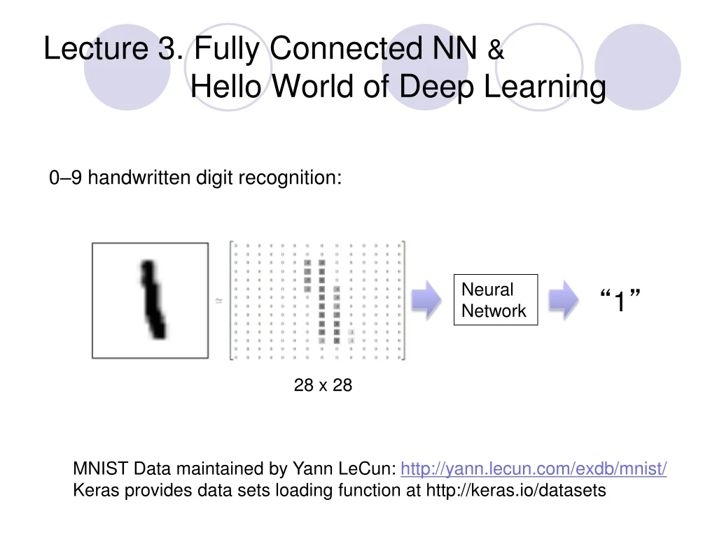
Lecture 3. Fully Connected NN & Hello World of Deep Learning. 0–9 handwritten digit recognition:. Neural Network. “ 1 ”. 28 x 28. MNIST Data maintained by Yann LeCun: http://yann.lecun.com/exdb/mnist/ Keras provides data sets loading function at http://keras.io/datasets.

E N D
Lecture 3. Fully Connected NN & Hello World of Deep Learning 0–9 handwritten digit recognition: Neural Network “1” 28 x 28 MNIST Data maintained by Yann LeCun: http://yann.lecun.com/exdb/mnist/ Keras provides data sets loading function at http://keras.io/datasets
Keras & Tensorflow • Interface of Tensorflow and Theano. • Francois Chollet, author of Keras is at Google, Keras will become Tensorflow API. • Documentation: http://keras.io. • Examples: https://github.com/fchollet/keras/tree/master/examples • Simple course on Tensorflow: https://docs.google.com/presentation/d/1zkmVGobdPfQgsjIw6gUqJsjB8wvv9uBdT7ZHdaCjZ7Q/edit#slide=id.p
Implementing in Keras 500 500 softmax y0 y1 y9 28x28 … Fully connected NN model = sequential() # layers are sequentially added model.add( Dense(input_dim=28*28, output_dim=500)) model.add(Activation(‘sigmoid’)) #: softplus, softsign,relu,tanh, hard_sigmoid model.add(Dense( output_dim = 500)) model.add (Activation(‘sigmoid’)) Model.add(Dense(output_dim=10)) Model.add(Activation(‘softmax’)) model.compile(loss=‘categorical_crossentropy’, optimizer=‘adam’, metrics=[‘accuracy’]) model.fit(x_train, y_train, batch_size=100, nb_epoch=20)
Training model.fit(x_train, y_train, batch_size=100, nb_epoch=20) numpy array 28 x 28 =784 10 Number of training examples Number of training examples
We do not really minimize total loss! Batch: parallel processing model.fit(x_train, y_train, batch_size=100, nb_epoch=20) • Randomly initialize network parameters • Pick the 1st batch NN x1 y1 y’1 L’ = l1 + l9+ … Update parameters l1 First batch NN x9 y9 y’9 • Pick the 2nd batch l9 …… L” = l2 + l16+ … Update parameters … NN x2 y2 y‘2 l2 • Until all batches have been picked 2nd batch NN x16 y16 y’16 one epoch l16 …… Repeat the above process
Speed Very large batch size can yield worse performance • Smaller batch size means more updates in one epoch • E.g. 50000 examples • batch size = 1, 50000 updates in one epoch • batch size = 10, 5000 updates in one epoch 166s 1 epoch 10 epochs 17s Batch size = 1 and 10, update the same amount of times in the same period. 166s Batch size = 10 is more stable, converge faster GTX 980 on MNIST with 50000 training examples 17s
Speed - Matrix Operation • Why is batching faster? One at a time: = = Batch by GPU, 2 at a time, 1/2 time cost Matrix operation =