Cooling
Cooling. Eric Prebys , FNAL. Stochastic Cooling (antiprotons or ions). Anti-protons are created by hitting a target with an energetic proton beam. Most of what’s created are pions , but a small fraction are anti- protons.


Cooling
E N D
Presentation Transcript
Cooling Eric Prebys, FNAL
Stochastic Cooling (antiprotons or ions) Anti-protons are created by hitting a target with an energetic proton beam. Most of what’s created are pions, but a small fraction are anti-protons. These are captured in a transport beam, but initially have a very large energy spread and transverse distribution. They must be “cooled” to be useful in collisions. We learned that electrons will naturally cool through synchrotron damping, but this doesn’t happen on a useful time scale for antiprotons, so at one time it was considered impossible to consider colliding protons with antiprotons, until.. Lecture 20 - Cooling
The basis of “stochastic cooling” is to detect the displacement at one point in the ring and provide a restoring kick at a second. For a single particle gain For a single particle, we could set g=1 and remove any deviation in a single turn. Lecture 20 - Cooling
However, we’re not dealing with single particles. If all particles retain their same relative longitudinal position, the Liouville’s Theorem tells us that the best we could do is correct the offset of the centroid – which is not cooling. We will therefore see that cooling will require the particles to “mix”. Consider an ensemble of particles sampling period bandwidth of pickup/kicker system Pickups measure the mean position, and act on all particles equally, so for the ith particle, the change in one turn is Lecture 20 - Cooling
Isolate one particle (dropping turn index), and write mean of all other particles Plugging this back in, we get If the samples are statistically independent (not true in general), then over many turns RMS of x distribution Cooling stochastic heating =“Schottky noise” Lecture 20 - Cooling
Average over all particles This is the change in the RMS for one turn, so sample Recall total want high bandwidth Lecture 20 - Cooling
Note, electrical thermal noise will heat the system. This is typically normalized to the statistical Schottky noise In our analysis, we assumed that he sample was statistically independent from turn to turn, which is clearly not the case. This technique works via “mixing”, the fact that particles of different momenta have different periods. In general, it will take M turns to completely renew the samle. variation in periods Recall that revolution frequency Lecture 20 - Cooling
The effect on the test particle will be the same, but the net effect will be to increase the net Schottky heating by a factor of M Electronic noise Mixing time (turns) The optimum gain is then the max of Example: Fermilab Debuncher Noise ~twice beam signal Lecture 20 - Cooling
“Stacking” and Longitudinal Cooling The operation of “stacking” (accumulating beam) and longitudinal cooling both rely on placing pickups in a dispersive region. In the Fermilab antiproton source, injected beam is decelerated onto the core orbit. injected beam “core” Because of the η slip factor, beam will only “see” RF tuned to its momentum, and so beam can be selectively decelerated onto the core. Lecture 20 - Cooling
Once the beam is stacked, then the pickup system can be used to “kick” the beam energy and cool longitudinally, in the same way that the beam was colled transversely. core “stacktail” injected beam Lecture 20 - Cooling
Electron Cooling Electron cooling works by injecting “cold electrons” into a beam of negative ions (antiprotons or other) and cooling them through momentum exchange. Layout ion beam electron gun electron decelerator and collector Want Lecture 20 - Cooling
The electrons act like a drag force on the ions. At low velocity, the ionization loss varies as The velocity spread of the electrons is dominated by the energy distribution out of the cathode. In the rest frame, motion is non-relativistic relative velocity Energy spread. Typically ~.5 eV Lecture 20 - Cooling
Longitudinal Electron Cooling The momentum and energy between the rest and lab frames are related by beta of frame For efficient cooling, we want So for low energy beams, large momentum spreads can be tolerated, but as energy grows, only small momentum spreads can be efficiently cooled. Lecture 20 - Cooling
Transverse Electron Cooling Again, we want We have gets less effective for large gamma Electron cooling involves large currents, so it’s generally necessary to recover the energy from the non-interacting electrons and reuse them”pelletron” Lecture 20 - Cooling
Electron Cooling in the Fermilab Recycler One of the highest energy and most successful electron cooling systems was in the Fermilab “Recycler” – an 8 GeV permanent storage ring which was used to store anti-protons for use in the Tevatron collider. pelletron .5 A “u-beam” Lecture 20 - Cooling
Ionization Cooling (Muons Only) Lecture 20 - Cooling • There has long been interest in the possibility of using muons to produce high energy interactions. They have two distinct advantages • Like electrons, the are point-like, so the entire beam energy is available to the interaction – in contrast to protons. • Because they are much heavier than electrons, synchrotron radiation does not become a serious issue until extremely high energies (10s or 100s or TeV). • Of course, they have one big disadvantage • They are unstable, with a lifetime of 2.2 μsec. • For this reason, traditional cooling methods are far to slow to be useful. • Don’t radiate enough for radiative damping • Don’t live long enough for stochastic cooling.
Principle of ionization cooling absorber accelerator As they accelerate back to their initial energy, the normalized emittance is therefore reduced (ie, adiabatic damping). Particles lose energy along their path. The position and angle do not change, so the un-normalized emittance remains constant; however, because the energy is lower, that means the normalized emittance has been reduced. Of course, there’s also heating from multiple scattering. so the change in the normalized emittance is heating from multiple scattering <0 cooling term Lecture 20 - Cooling
Use define dE/dx as energy loss, which changes sign heating cooling term Lecture 20 - Cooling
From our discussion of multiple scattering, we have The equilibrium emittance is • Want • small βx • large X0low Z • H2? • Li? ~independent of material drops with Z Lecture 20 - Cooling