Supernova relic neutrinos
670 likes | 881 Vues
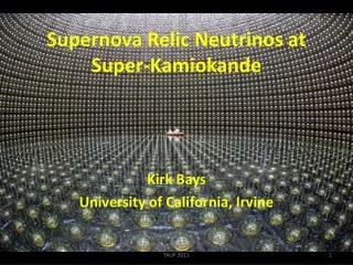
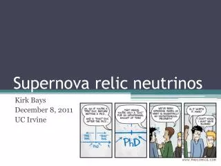
Supernova relic neutrinos. Kirk Bays December 8, 2011 UC Irvine. OUTLINE. 1) Theory and background: supernovae, SN neutrinos, and what has come before 2) Super-K: what is it, how does it work 3) Tools: software used to study neutrinos 4) Event selection: cut out the backgrounds!

Supernova relic neutrinos
E N D
Presentation Transcript
Supernova relic neutrinos Kirk Bays December 8, 2011 UC Irvine
OUTLINE. • 1)Theory and background: supernovae, SN neutrinos, and what has come before • 2)Super-K: what is it, how does it work • 3) Tools: software used to study neutrinos • 4) Event selection: cut out the backgrounds! • 5) Remaining backgrounds: understand, model • 6) Analysis methodology: fits fitsfits • 7) Results: getting this is the whole point • 8) Discussion: What does it all mean?
1: Theory and background www.smbc-comics.com
Supernovae • Stars are fueled by nuclear fusion • Mostly fuse H into He, as the universe began full of hydrogen • When hydrogen is used up, it collapses • If the star is massive enough, begins fusing He, becomes layered • Stars > ~8 solar masses can fuse elements all the way to iron • Iron doesn’t fuse, and without fusion the core collapses on itself • This makes the core super-hot and dense; also the collapse rebounds when it becomes dense enough to hit neutron-neutron interactions • Rebound shock + emissions from superhot core = supernova
Supernova neutrinos • Released E: En~99%, Ekinetic~1%, Elight~0.1% • As the core collapses, high temperature and pressure make electron capture favorable: • e + p n + ne (neutronization burst, ~1044 J, ~10 ms, ne) • After the rebound, the core is superheated (~100 billion K), and releases neutrino-antineutrino pairs of all flavors equally. These neutrinos are trapped by the collapsed core, and leak out; they also fuel the explosion (rebound not enough alone) (thermal burst, ~1046 J ,~10 s, all flavors) more neutrons Livermore numerical model ApJ 496 (1998) 216 CC+NC NC only
SN 1987A 2140 tons SN neutrino bursts • SN1987A: first neutrinos definitely seen from farther than the sun • Galactic supernova: ~3/century 6800 tons in SK today: ~10k events Gal. center 200 tons scintillator arXiv:hep-ph/0412046v2
The DSNB • Even though we would not see the n burst from far away supernovae, the neutrinos from all supernovae in the history of the universe combined should be a diffuse, detectable signal. • This is called the Diffuse Supernova Neutrino Background (DSNB), or Supernova Relic Neutrinos (SRN, `relics’). These terms are interchangeable. • This signal has never been seen. • Many theorists have constructed models of the DSNB • Only a few events/year are expected at SK. This is a rare signal Cosmic Gas Infall – Malaney - R. A. Malaney, AstroparticlePhysics 7, 125 (1997) Chemicalevolution - D. H. Hartmann and S. E.Woosley, Astroparticle Physics 7, 137 (1997) Heavy Metal Abundance - M. Kaplinghat, G. Steigman, and T. P. Walker, Phys. Rev. D 62, 043001 (2000) Large Mixing Angle - S. Ando, K. Sato, and T. Totani, Astroparticle Physics 18, 307 (2003) (updated NNN05) Failed Supernova - C. Lunardini, Phys. Rev. Lett. 102, 231101 (2009) (assume Failed SN rate = 22%, EoS = Lattimer-Swesty, and survival probability = 68%.) 6/4 MeV FD spectrum - S. Horiuchi, J. F. Beacom, and E. Dwek, Phys. Rev. D 79, 083013 (2009).
= DSNB flux • z = red shift parameter • RSN = CC SN rate Anatomy of a DSNB model RSF = star formation rate • Main ingredients: star formation history, spectrum • Star formation history well measured in recent years • As most SN ns thermally produced, use Fermi-Dirac spectrum: • Leaves 2 free parameters: = n luminosity, T = n temperature • Downside: FD imperfect description S. Horiuchi, J. F. Beacom, and E. Dwek, Phys. Rev. D 79, 083013 (2009)
Phys. Rev. Lett. 90, 061101 (2003) Current knowledge 90% CL SRN • In 2003, SK published a paper detailing the first SRN search at SK • Final 90% CL flux limit: • 1.2 n cm-2s-119.3<En<83.3 MeV • 100x previous limit • Most stringent limit ever • Methodology: implement cuts to remove most backgrounds • Model remaining backgrounds • c2 fit (SNR + 2 backgrounds) • No indication for SNR events • Many theories predict the SRN signal to be on the edge of this limit • I have now improved this study significantly ne CC decay e’s from `invisible’ nm m’s ‘Our best estimate for the flux at Super-K is slightly below, but very close to the current SK upper limit. …We estimate that the SRN background should be detected (at 1σ) at Super-K with a total of about 9 years (including the existing 4 years) of data.’ L. Strigari, M. Kaplinghat, G. Steigman, T. Walker, The Supernova Relic Neutrino Backgrounds at KamLAND and Super-Kamiokande, JCAP 0403 (2004) 007
Water system: filtration, degasification, water flow water entering tank 18.2 MΩ*cm leaving tank 11 MΩ*cm 35-70 tons/hour water flow Super-Kamiokande Kamiokaneutrino detection experiment 50 ktons ‘Inner Detector’, ID • ~11,150 inward facing photomultiplier tubes • single photon sensitivity • ~40% surface coverage 41.4 m • ‘Outer Detector’, OD • Optically separate from ID • 1885 outward facing PMTs underground 2700 m.w.e. 39.3 m 26 Helmholtz coils reduce Earth’s magnetic field by factor of 9 ID fiducial volume two meters from PMTs; 32.5 ktons -> 22.5 Ktons • Radon system: • 99.98% effective at reducing radon • reduces background, worker health
Detector History SK-I (40% coverage, 1497 live days 11,146 PMTs) • April 1 1996: begin data taking • July 15 2001: stop for maintenance • Nov 11 2001: Accident destroys ~60% of PMTs while refilling • Oct 8 2002: Masatoshi Koshiba awarded Nobel Prize in physics (25%) • Dec 6 2002: Surviving PMTs repositioned, start data taking again • Feb 2003: First SRN paper published • Late 2005: begin full repair • 2006: Kirk joins the team! • June 2006: Full repairs complete, start new data taking • Aug 2008: Full electronics upgrade • Sep 2008: continue data taking • Nov 2011: SRN paper submitted to PRD! SK-II (19% coverage, 794 live days) SK-III (40% coverage, 562 live days) SK-IV (40% coverage)
Physics in SK • High energy particles interact in the water, create light via the well known Cherenkov effect • For DSNB events, inverse beta decay is by far the dominant mode AstroparticlePhysics 3 (1995) 367-376 Event rate (/yr/MeV) arXiv:hep-ph/0412046v2 e- kinetic E (MeV)
.3 p.e. Triggering, DAQ • Dark noise: 3-5 KHz. • PMT timing resolution ~3 ns • Lower trigger thresholds can detect lower energy events • Limited by computing power • 2 channels/PMT keep detector mostly dead-time free • SK-IV electronics different, not discussed here -11 mV The Super-Kamiokande Detector The Super-Kamiokande Collaboration, Nucl. Instrum. Meth. A501(2003)418-462 Final trigger records data in 1.3 μs range (one ‘event’)
Calibration • LINAC: • Most important calibration source • Old medical linear accelerator, on site • Shoots mono-energetic electrons ( 5 – 18 MeV) into known positions • Energy known to within 20 KeV • Primary calibration of absolute energy scale (accurate to within 1%) • Also useful for energy resolution, angular resolution, spatial resolution • Xe/laser source and scintillator ball: • Helps fine tune high voltage to regulate individual PMT gain • N2 laser and diffuser ball: • Relative PMT timing, ‘tq map’ • Deuterium-tritium neutron generator (DT): • double check absolute energy scale, trigger efficiency • Decay electrons: • determines water transparency for LE group, stability of energy scale Nucl. Instrum. Meth. A501(2003)418-462
atmospheric Signals in SK • Atmospheric neutrinos up to TeV • Reactor, solar, relic ns (all < 21 MeV) • Cosmic ray muons (~2Hz) • Spallation (<24 MeV) • Stopping muon decay electrons • …. solar
e-/e+ reconstruction Vertex fitting: • Electrons travel ~10 cm before stopping • This is on the order of resolution; can consider a point-like event • Reconstructed with BONSAI (by Michael) • uses only the PMT timing information • fits a dark noise component • constructs likelihood, compares to likelihood derived from LINAC data • best resolution of all SK fitters Energy fit: • Charge determination for PMTs poor at low levels, assume 1 p.e. per hit • Takes into account dark noise, water transparency, geometry, occupancy correction • E resolution ~10% @ 18 MeV Direction Fit: • Likelihood fit; resolution ~20 degrees • Vertex, direction, and energy reconstruction tools are the same as used for the long established SK solar analyses • All energies quoted are total electron equivalent energy M.B. Smy, Low Energy Challenges in Super- Kamiokande-III, Nuc. Phy. B, 168, pg 118-121 (2007)
e p Cherenkov angle • Reconstructing the Cherenkov angle important for particle ID • Reconstruction algorithm takes 3 hit PMTs, forms a cone with an opening angle; looks at all 3-hit combinations, fits to peak of distribution • Events with multiple particles, gammas, emit light more isotropically; algorithm biases these to high angles • Width of distribution also can be used to discriminate e’svsp’s
Muon fitting dE/dx • Main muon fitter name Muboy • Better track resolution than fitter used in 2003 (entry point resolution ~100cm, direction resolution ~6 deg.) • Can categorize muons by type: • Single through-going (~82%) • Stopping (~7%) • Multiple muons (2 types) (~7%) • Corner clipper (~4%) • Can’t fit (<1%) • We can make a dE/dx distribution of muon track based on Muboy fit • Also developed an alternate fitter (Brute Force Fitter, BFF) for when Muboy fails; can refit ~75% of misfit singles get dE/dx using timing info assume light travels at v=c/n and muon at v = c; determine where along track light originated quadratic Eqn w/ 2 solutions, keep both Take into account corrections based on water transparency, coverage
Multiple Coulomb scattering • Electrons can multiple Coulomb scatter in the detector • It can be useful to estimate how much an electron scatters • Select PMT, construct cone w/ 42o angle from vertex to PMT; intersection points of cones gives unit vectors • Do this for all combination of 2 hit PMTs • Vector adding all the direction unit vectors/ # unit vectors gives a value between 0 (completely unaligned) to 1 (all perfectly aligned) • This value is used as a `goodness’; estimates multiple Coulomb scattering Best Fit Direction
First reduction reduces data volume by ~2 orders of magnitude • SK records immense amount of data • Much of this can be removed with some simple cuts • Eliminates major backgrounds and makes the rest of the data more manageable • Similar to solar first reduction remove: • OD triggered events • > 2,000 p.e. (1,000 SK-II) • > 800 hit tubes (400 SK-II) • Calibration events • Outside fiducial volume • < 16 or > 90 MeV • Electronics noise muons
spallation products expected in SK Spallation • Even at 2700 m.w.e., cosmic ray muons enter detector at ~2Hz • The muons can spall on oxygen nuclei, create radioactive products whose decays (mostly beta decays) can mimic SRNs • Spallation occurs < 24 MeV; lower the energy, the more spallation • Dominant low energy background • Want final sample spallation free, as it is hard to model; determines analysis lower energy threshold • Spallation eliminated by correlating to preceding muons • Spallation cut in 2003: • lose 36% signal efficiency • uses cut tuned for solar • only down to 18 MeV
4 variable likelihood cut • The 4 variables: • dlLongitudinal • dt • dlTransverse • Qpeak • Muboy: better resolution μ fit • Tune separate likelihoods for each muon type (single, multiple, stopping) μentry point Spallation Cut μ track dlLongitudinal new where peak of dE/dxplot occurs old likelihood • Correlate events to all muons within previous 30 seconds • Muons within 30 seconds after relic candidates make final sample • Data sample – random sample = spall sample • Make likelihoods (PDFs) for each variable dlTransverse Relic Candidate QPeak= sum of charge in window dE/dx p.e.’s spallation expected here distance along muon track (50 cm bins)
Spallation cut • SK-I/III cut combined; SK-II different • Additional tracks for multiple muons have own special PDFs • If Muboy fails fit, check BFF Examples for SK-I/III singles QPEAK p.e. (x 103)
2003 Old cut 18 < E < 34: 36% signal ineff. New Cut (SK-I/III): 16 < E < 18 MeV: 18% signal ineff. 18 < E < 24 MeV: 9% signal ineff. New Cut (SK-II): 17.5 < E < 20 MeV: 24% signal ineff. 20.0 < E < 26 MeV: 12% signal ineff. Spallation cut • Improvements allow lowering of energy threshold • Requires 2-stage cut • Inefficiency calculated for all detector (position dependent) • SRN MC vertex distribution used to get overall inefficiency
SolarνEvents energy resolution for an event of energy: 16 MeV 18 MeV pp 7Be • Solar 8B and hep neutrinos are a SRN background (hep at 18 MeV, and both at 16 MeV, because of energy resolution) • Cut criteria is optimized using 8B/hep MC • 2003: 1 cut < 34 MeV • New cut is now energy dependent, tuned in 1 MeV bins pep 8B hep 16 18 e recoil energy (total) (MeV)
Solar n cut combined MSgood< 0.4 0.4 < MSgood< 0.5 0.5 < MSgood< 0.6 0.6 < MSgood • Solar events cut using qsun • cos(qsun) = 1 if reconstructed direction matches sun • 2003 cut: remove cos(qsun)>0.87 for all events E < 34 MeV • ~15 degree resolution from the physics; multiple scattering of electron makes resolution worse • Use multiple Coulomb scattering estimator `MSgood’ to improve efficiency by using a separate cut for each MSgood bin, for each 1 MeV energy bin integrated cos(θsun)
Solar n cut Significance: e = cut efficiency k = cut effectiveness Nsolar = # solar eva = # background ev k* Nsolar = # solar events after cut applied significance • Determine optimal cut points using `significance’ function • Significance assumes dominant decay-e background only, represents signal/sqrt(background) • Number of solar events modeled using MC spectrum, normalized using data < 16 MeV • SK-I/III solar cut same, SK-II different cos(θsun)
Incoming event cut remaining removed (2003) recovered (now) • Large amounts of background exists near the walls • Much is removed by the fiducial volume cut; some survives • The deff variable can help discriminate these events without the inefficiency of removing more volume • Incoming events will have smaller deff; also incorrectly fit events that are really near the wall tend to have small deff • Retune SK-I to increase efficiency • SK-II and SK-III separately tuned; not enough statistics for energy dependent tuning
More cuts • multiple timing peak • multiple rings • Pion cut • uses width of 3-hit combination distributions • OD correlated • check hit ID tubes for correlations in time and space to OD hit tubs, even if no OD trigger • Pre-post activity • remove events +/- 50 ms; for SLE events require 5 m correlation
Efficiency • Efficiency greatly increased from 2003 • With lower energy threshold, efficiency is 87% greater in SK-I • Including new SK-II and SK-III data, efficiency is increased by 227% • Sensitivity improvement: • sqrt(3.3) 80% better sensitivity • Systematic errors calculated on efficiency; mostly from studying LINAC data vs LINAC MC SK-I final efficiency (sys error)
5. Remaining backgrounds www.smbc-comics.com
After cuts, want final sample `free’ of these backgrounds (spallation, solar, pions, decay electrons, etc) • Check many distributions to try and determine if this is true • Due to low statistics, very difficult to be sure backgrounds completely gone; can only so no statistically significant amount remaining • Estimated remaining in SK-I/II/III • Spall: < 4 • Solar: < 2 • deff cut: < 2 • Any remaining background likely to make limit more conservative Cut backgrounds final sample data random sample single muons dt (s)
SK-I backgrounds Remaining Backgrounds # events estimated in SK-I all SRN cuts applied • Final sample still mostly backgrounds, from atmospheric n interactions; modeled w/ MC • 1) nm CC events • muons from atmospheric nm’s can be sub-Cherenkov; their decay electrons mimic SRNs • modeled with decay electrons • 2)ne CC events • indistinguishable from SRNs • 3)NC elastic • low energy mostly • 4)m/p events • combination of muons and pions remaining after cuts Backgrounds 1) and 2) were considered in the 2003 study. Backgrounds 3) and 4) are new!
Low angle events Signal region NC region p ne 42o n e+ 25-45o μ, π N n reconstructed angle near 90o n (invisible) • SRN events expected (98% SK-I) in the central, signal region (38-50o) • ‘Sidebands’ previously ignored • Now that we consider new background channels, sidebands useful • NC elastic events occur at high C. angles • m/p events occur at low C. angles • Sidebands help normalize new backgrounds in signal region not used
Maximum likelihood fit • 2003 study used binned c2 to fit final sample • Found that changing the binning could change answer (up to 20%) • Instead use unbinned maximum likelihood fit • Fit all 4 backgrounds in all three Cherenkov regions, (for SK-I/II/III each), make PDFs • Also make PDFs for all relic models • Loops over all combinations of events, maximize likelihood F is the PDF for a particular channel; E is the event energy; c is the magnitude of each channel; irepresents a particular event, and j represents a channel (SRN + 4 backgrounds)
Make likelihood function of amount of distortion Systematic errors L(r) L’(r,e) Then sum all combinations of distorted likelihoods, weighed by Gaussian envelope • Many systematics considered, were not considered in 2003 • All the systematics operate by distorting the likelihood • 1) Energy resolution/ E scale • Error on MC • considered independent • distortions added in quadrature • 2) Energy independent efficiency • Systematic from cut reduction • Also cross section, FV errors • Spectral shape systematics • Apply very conservative errors to NC elastic, ne CC channels. • decay electron background from data, no error; neglect m/p example: E res/scale decay-e SRN L =c1PDF1(E) + c2p2(E) …. apply E res/scale distortion to PDF1: L(e) =c1PDF1(E,e) + c2p2(E) …. sum with weights for new likelihood
Fit results Ando et al.’s LMA model; SRN best fit 0
Fit results • SK-II and SK-III give a positive fit for SRN signal • This positive indication is not significant
LMA = Ando et al (LMA model) HMA = Kaplinghat, Steigman, Walker (heavy metal abundance) CGI = Malaney (cosmic gas infall) FS = Lunardini (failed SN model) CE = Hartmann/Woosley (chemical evolution) 4/6MeV = Horiuchi et al n temp IMB 1987A allowed Kamiokande1987A allowed
COMPARISON TO PUBLISHED LIMIT 2003 now
What’s next for SRNs? • Analysis already includes 176 ton-years of data • Now highly optimized • Further improvements will be slow • There is some hope for background reduction in SK-IV with new electronics (neutron tagging) • Still, it is unlikely that a discovery can be made at SK in the near future • Gd doping could be a solution • neutron tagging allows background reductions • removes most spallation, lower energy threshold • Otherwise wait for next generation detectors