Download
1 / 27
270 likes | 408 Vues
Some Aspects of Mean Field Dynamo Theory. David Hughes Department of Applied Mathematics University of Leeds. The Sun’s Global Magnetic Field. Ca II emission Extreme ultra-violet. Temporal variation of sunspots.

E N D
Some Aspects of Mean Field Dynamo Theory David Hughes Department of Applied Mathematics University of Leeds ICTP Trieste
The Sun’s Global Magnetic Field Ca II emission Extreme ultra-violet ICTP Trieste
Temporal variation of sunspots Number of sunspots varies cyclically with an approximately 11 year cycle. Latitudinal location of spots varies with time – leading to butterfly diagram. Sunspots typically appear as bipolar pairs. Polarity of sunspots opposite in each hemisphere Polarity of magnetic field reverses every 11 years. 22 year magnetic cycle. Known as Hale’s polarity laws. ICTP Trieste
The Solar Dynamo Now almost universally believed that the solar magnetic field is maintained by some sort of dynamo mechanism, in which the field is regenerated by inductive motions of the electrically conducting plasma. The precise site of the dynamo is still a matter of some debate – though is certainly in all, or part, of the convection zone and, possibly, in the region of overshoot into the radiative zone. Dynamo theory deals with the regeneration of magnetic fields in an electrically conducting fluid or gas – nearly always through the equations of magnetohydrodynamics (MHD). The vast majority of the modelling of astrophysical dynamos has been performed within the framework of mean field electrodynamics. ICTP Trieste
Starting point is the magnetic induction equation of MHD: where B is the magnetic field, u is the fluid velocity and η is the magnetic diffusivity (assumed constant for simplicity). Assume scale separation between large- and small-scale field and flow: In dimensionless units: where B and U vary on some large length scale L, and u and b vary on a much smaller scale l. where averages are taken over some intermediate scale l « a « L. Kinematic Mean Field Theory ICTP Trieste
This equation is exact, but is only useful if we can relate to For simplicity, ignore large-scale flow, for the moment. Induction equation for mean field: where mean emf is ICTP Trieste
Consider the induction equation for the fluctuating field: where Traditional approach is to assume that the fluctuating field is driven solely by the large-scale magnetic field. i.e. in the absence of B0 the fluctuating field decays. i.e. No small-scale dynamo (and hence between and Under this assumption, the relation between ) is linear and homogeneous. and ICTP Trieste
Postulate an expansion of the form: where αij and βijk are pseudo-tensors. Simplest case is that of isotropic turbulence, for which αij = αδij and βijk = βεijk. Then mean induction equation becomes: α: regenerative term, responsible for large-scale dynamo action. Since is a polar vector whereas Bis an axial vector then α can be non-zero only for turbulence lacking reflexional symmetry (i.e. possessing handedness). The simplest measure of the lack of reflexional symmetry is the helicity of the flow, β: turbulent diffusivity. ICTP Trieste
For the former (assuming isotropy): Correlations between u and b have been replaced by correlations between u and w. For the latter: where F(k,ω) is the helicity spectrum function. Analytic progress possible if we neglect the G term (“first order smoothing”). This can be done if either the correlation time of the turbulence t or Rm is small. These results suggest a clear link between α and helicity. ICTP Trieste
Mean field dynamo theory is very user friendly. With a judicial choice of α and β (and differential rotation ω) it is possible to reproduce a whole range of observed astrophysical magnetic fields. e.g. butterfly diagrams for dipolar and quadrupolar fields: (Tobias 1996) Mean Field Theory – Applications A dynamo can be thought of as a mechanism for “closing the loop” between poloidal and toroidal fields. Velocity shear (differential rotation) naturally generates toroidal from poloidal field. The α-effect of mean field electrodynamics can complete the cycle and regenerate poloidal from toroidal field. ICTP Trieste
Crucial questions Mean field dynamo models “work well” – and so, at some level, capture what is going on with cosmical magnetic fields. However, all our ideas come from consideration of flows with either very short correlation times or with very small values of Rm. What happens in conventional MHD turbulence with O(1) correlation times and Rm >> 1? • We still do not fully understand the detailed micro-physics underlying the • coefficients α, β, etc. – maybe not even in the kinematic regime. • What happens when the fluctuating field may exist of its own accord, independent of the mean field? • What is the spectrum of the magnetic field generated? Is the magnetic energy dominated by the small scale field? 3. What is the role of the Lorentz force on the transport coefficients α and β? How weak must the large-scale field be in order for it to be dynamically insignificant? Dependence on Rm? We shall address some of these via an idealised model. ICTP Trieste
Rotating turbulent convection T0 Ω g T0 + ΔT Cattaneo & Hughes 2005 Anti-symmetric helicity distribution anti-symmetric α-effect. Maximum relative helicity ~ 1/3. Boussinesq convection. Boundary conditions: impermeable, stress-free, fixed temperature, perfect electrical conductor. Taylor number, Ta = 4Ω2d4/ν2 = 5 x 10⁵, Prandtl number Pr = ν/κ = 1, Magnetic Prandtl number Pm = ν/η = 5. Critical Rayleigh number = 59 008. ICTP Trieste
Ra = 500,000 Ra = 70,000 Ra = 150,000 Relative Helicity Temperature near upper boundary (5 x 5 x 1 box) ICTP Trieste
Ra = 106 Box size: 10 x 10 x 1, Resolution: 512 x 512 x 97 Snapshot of temperature. No imposed mean magnetic field. Growth of magnetic energy takes place on an advective (i.e. fast) timescale. A Potentially Large-Scale Dynamo Driven by Rotating Convection ICTP Trieste
Bx No evidence of significant energy in the large scales – either in the kinematic eigenfunction or in the subsequent nonlinear evolution. Picture entirely consistent with an extremely feeble α-effect. Healthy small-scale dynamo; feeble large-scale dynamo. ICTP Trieste
Enlargement of the above. α and its cumulative average versus time. Imposed horizontal field of strength B0 = 10. ICTP Trieste
time time Turbulent α-effect with no small-scale dynamo Ra = 150 000 Temperature on a horizontal slice close to the upper boundary. Ra = 150,000. No dynamo at this Rayleigh number – but still an α-effect. Mean field of unit magnitude imposed in x-direction. Self-consistent dynamo action sets in at Ra 180,000. ICTP Trieste
e.m.f. and time-average of e.m.f. Ra = 150,000 Imposed Bx = 1. Imposed field extremely weak – kinematic regime. time time time ICTP Trieste
Cumulative time average of the e.m.f. Not fantastic convergence. α – the ratio of e.m.f. to applied magnetic field – is very small. At first sight this appears to be consistent with the idea of α-effect suppression. However, the field here is too weak for this. Thus it appears that the α-effect here is not turbulent (i.e. fast), but diffusive (i.e. slow). ICTP Trieste
Changing Pm The α-effect here is inversely proportional to Pm (i.e. proportional to η). It is therefore not turbulent (i.e. fast), but diffusive (i.e. slow). ICTP Trieste
Jones & Roberts work with the Ekman number E and a modified Rayleigh number RaW Relation to the work of Jones & Roberts (2000) Similar model – dynamo driven by rotating Boussinesq convection – but with the following differences: • Infinite Prandtl number • Different boundary conditions • (i) No-slip velocity conditions • (ii) Magnetic field matches onto a potential field. • Smaller box size ICTP Trieste
Temperature contours for mildly supercritical convection – no field. ICTP Trieste
Magnetic energy vs time for (a) RaΩ = 500, q = 5, E = 0.001 (b) RaΩ = 1000, q = 1, E = 0.001 ICTP Trieste
The Influence of Box Size for the Idealised Problem Ra = 80 000 Temperature contours: aspect ratio = 0.5 u2 = 330 3 components of e.m.f. vs time, calculated over upper and lower half-spaces. αxx 8.5 ICTP Trieste
Kinetic Energy Aspect ratio = 1 time αxx 1.6 ICTP Trieste
Conclusions • Rotating convection is a natural way of producing a helical flow, even at • high values of Ra, when the flow is turbulent. However, the simple ideas derived • for small correlation time or small Rm do not carry over to turbulent flows • with an O(1) value ofτ and a high value of Rm. • 2. The α-effect driven by rotating, “turbulent” convection seems to be • (a) hard to measure – wildly fluctuating signal in time, even after averaging over • many convective cells. Convergence is painfully slow. • (b) feeble (i.e. diffusive); • 3. Given (a), what meaning should we give to the α-effect in this case? ICTP Trieste