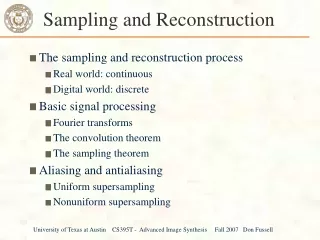
Sampling and Reconstruction
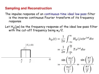
Sampling and Reconstruction The impulse response of an continuous-time ideal low pass filter is the inverse continuous Fourier transform of its frequency response Let H lp (jw) be the frequency response of the ideal low-pass filter with the cut-off frequency being w s /2.


Sampling and Reconstruction
E N D
Presentation Transcript
Sampling and Reconstruction The impulse response of an continuous-time ideal low pass filter is the inverse continuous Fourier transform of its frequency response Let Hlp(jw) be the frequency response of the ideal low-pass filter with the cut-off frequency being ws/2.
Remember that when we sample a continuous band-limited signal satisfying the sampling theorem, then the signal can be reconstructed by ideal low-pass filtering.
The sampled continuous-time signal can be represented by an impulse train: Note that when we input the impulse function (t) into the ideal low-pass filter, its output is its impulse response When we input xs(t) to an ideal low-pass filter, the output shall be • It shows that how the continuous-time signal can be reconstructed by interpolating the discrete-time signal x[n].
Properties: hr(0) = 1; hr(nT) = 0 for n=1, 2, …; It follows that xr(mT) = xc(mT), for all integer m. The form sin(t)/t is referred to as a sinc function. So, the interpolant of ideal low-pass function is a sinc function.
Ideal discrete-to-continuous (D/C) converter • It defines an ideal system for reconstructing a bandlimited signal from a sequence of samples.
Ideal low pass filter is non-causal • Since its impulse response is not zero when n<0. Ideal low pass filter can not be realized • It can not be implemented by using any difference equations. Hence, in practice, we need to design filters that can be implemented by difference equations, to approximate ideal filters.
Z-Transform • Discrete-time Fourier Transform • z-transform: polynomial representation of a sequence
Z-Transform (continue) • Z-transform operator: • The z-transform operator is seen to transform the sequence x[n] into the function X{z}, where z is a continuous complex variable. • From time domain (or space domain, n-domain) to the z-domain
Bilateral vs. Unilateral • Two sided or bilateral z-transform • Unilateral z-transform
Relationship to the Fourier Transform • If we replace the complex variable z in the z-transform by ejw, then the z-transform reduces to the Fourier transform. • The Fourier transform is simply the z-transform when evaluating X(z) only in a unit circle in the z-plane. • From another point of view, we can express the complex variable z in the polar form as z = rejw. With z expressed in this form,
Relationship to the Fourier Transform (continue) • In this sense, the z-transform can be interpreted as the Fourier transform of the product of the original sequence x[n] and the exponential sequence rn. • For r=1, the z-transform reduces to the Fourier transform. The unit circle in the complex z plane
Relationship to the Fourier Transform (continue) • Beginning at z = 1 (i.e., w = 0) through z = j(i.e., w = /2) to z = 1 (i.e., w =), we obtain the Fourier transform from 0 w . • Continuing around the unit circle in the z-plane corresponds to examining the Fourier transform from w = to w = 2. • Fourier transform is usually displayed on a linear frequency axis. Interpreting the Fourier transform as the z-transform on the unit circle in the z-plane corresponds conceptually to wrapping the linear frequency axis around the unit circle.
Convergence Region of Z-transform • The sum of the series may not be converge for all z. • Region of convergence (ROC) • Since the z-transform can be interpreted as the Fourier transform of the product of the original sequence x[n] and the exponential sequence rn, it is possible for the z-transform to converge even if the Fourier transform does not. • Eg., x[n] = u[n] is absolutely summable if r>1. This means that the z-transform for the unit step exists with ROC |z|>1.
ROC of Z-transform • In fact, convergence of the power series X(z) depends only on |z|. • If some value of z, say z = z1, is in the ROC, then all values of z on the circle defined by |z|=| z1| will also be in the ROC. • Thus the ROC will consist of a ring in the z-plane.
Analytic Function and ROC • The z-transform is a Laurent series of z. • A number of theorems from the complex-variable theory can be employed to study the z-transform. • A Laurent series, and therefore the z-transform, represents an analytic function at every point inside the region of convergence. • Hence, the z-transform and all its derivatives exist and must be continuous functions of z with the ROC. • This implies that if the ROC includes the unit circle, the Fourier transform and all its derivatives with respect to w must be continuous function of w.
Z-transform and Linear Systems • First, we analyze the Z-transform of a causal FIR system • The impulse response is • Take the z-transform on both sides
Z-transform of Causal FIR System (continue) • Thus, the z-transform of the output of a FIR system is the product of the z-transform of the input signal and the z-transform of the impulse response.
y[n] Y(z) x[n] X(z) h[n] H(z) Z-transform of Causal FIR System (continue) • H(z) is called the system function (or transfer function) of a (FIR) LTI system.
V(z) Y(z) Y(z) Y(z) X(z) X(z) H2(z) H1(z) H1(z) V(z) H2(z) Y(z) X(z) H1(z)H2(z) Multiplication Rule of Cascading System
Example • Consider the FIR system y[n] = 6x[n] 5x[n1] + x[n2] • The z-transform system function is
z1 Delay of one Sample • Consider the FIR system y[n] = x[n1], i.e., the one-sample-delay system. • The z-transform system function is
zk Delay of k Samples • Similarly, the FIR system y[n] = x[nk], i.e., the k-sample-delay system, is the z-transform of the impulse response [n k].
+ + + + + + + + b0 b0 TD TD TD z1 z1 z1 x[n] x[n] y[n] y[n] b1 b2 bM bM b2 b1 x[n-1] x[n-1] x[n-2] x[n-2] x[n-M] x[n-M] System Diagram of A Causal FIR System • The signal-flow graph of a causal FIR system can be re-represented by z-transforms.
Z-transform of General Difference Equation (IIR system) • Remember that the general form of a linear constant-coefficient difference equation is • When a0is normalized to a0= 1, the system diagram can be shown as below for alln
+ + + + + + + + x[n] y[n] b0 TD TD TD TD TD TD bM b1 b2 a1 a2 aN y[n-1] x[n-1] x[n-2] y[n-2] y[n-N] x[n-M] Review of Linear Constant-coefficient Difference Equation
+ + + + + + + + X(z) Y(z) b0 z1 z1 z1 z1 z1 z1 b1 bM b2 a1 aN a2 Z-transform of Linear Constant-coefficient Difference Equation • The signal-flow graph of difference equations represented by z-transforms.
Z-transform of Difference Equation (continue) • From the signal-flow graph, • Thus, • We have
Z-transform of Difference Equation (continue) • Let • H(z) is called the system function of the LTI system defined by the linear constant-coefficient difference equation. • The multiplication rule still holds: Y(z) = H(z)X(z), i.e., Z{y[n]} = H(z)Z{x[n]}. • The system function of a difference equation (or a generally IIR system) is a rational formX(z) = P(z)/Q(z). • Since LTI systems are often realized by difference equations, the rational form is the most common and useful for z-transforms.
Z-transform of Difference Equation (continue) • When ak = 0 for k = 1 … N, the difference equation degenerates to a FIR system we have investigated before. • It can still be represented by a rational form of the variable z as
System Function and Impulse Response • When the input x[n] = [n], the z-transform of the impulse response satisfies the following equation: Z{h[n]} = H(z)Z{[n]}. • Since the z-transform of the unit impulse [n] is equal to one, we have Z{h[n]} = H(z) • That is, the system function H(z) is the z-transform of the impulse response h[n].
Z-transform vs. Convolution • Convolution • Take the z-transform on both sides:
Z-transform vs. Convolution (con’t) Time domain convolution implies Z-domain multiplication
Y(z) (= H(z)X(z)) Z-transform Fourier transform X(z) H(z)/H(ejw) X(ejw) Y(ejw) (= H(ejw)X(ejw)) System Function and Impulse Response (continue) • Generally, for a linear system, y[n] = T{x[n]} • it can be shown that Y{z} = H(z)X(z). where H(z), the system function, is the z-transform of the impulse response of this system T{}. • Also, cascading of systems becomes multiplication of system function under z-transforms.
Poles and Zeros • Pole: • The pole of a z-transform X(z) are the values of z for which X(z)= . • Zero: • The zero of a z-transform X(z) are the values of z for which X(z)=0. • When X(z) = P(z)/Q(z) is a rational form, and both P(z) and Q(z) are polynomials of z, the poles of are the roots of Q(z), and the zeros are the roots of P(z), respectively.
Examples • Zeros of a system function • The system function of the FIR system y[n] = 6x[n] 5x[n1] + x[n2] has been shown as • The zeros of this system are 1/3 and 1/2, and the pole is 0. • Since 0 and 0 are double roots of Q(z), the pole is a second-order pole.
Example: Finite-length Sequence (FIR System) Given Then There are the N roots of zN = aN, zk = aej(2k/N). The root of k = 0 cancels the pole at z=a. Thus there are N1 zeros, zk = aej(2k/N), k = 1 …N, and a (N1)th order pole at zero.
Example: Right-sided Exponential Sequence • Right-sided sequence: • A discrete-time signal is right-sided if it is nonzero only for n0. • Consider the signal x[n] = anu[n]. • For convergent X(z), we need • Thus, the ROC is the range of values of z for which |az1| < 1 or, equivalently, |z| > a.
: zeros : poles Gray region: ROC Example: Right-sided Exponential Sequence (continue) • By sum of power series, • There is one zero, at z=0, and one pole, at z=a.
Example: Left-sided Exponential Sequence • Left-sided sequence: • A discrete-time signal is left-sided if it is nonzero only for n 1. • Consider the signal x[n] = anu[n1]. • If |az1| < 1 or, equivalently, |z| < a, the sum converges.
Example: Left-sided Exponential Sequence (continue) • By sum of power series, • There is one zero, at z=0, and one pole, at z=a. The pole-zero plot and the algebraic expression of the system function are the same as those in the previous example, but the ROC is different.
Hence, to uniquely identify a sequence from its z-transform, we have to specify additionally the ROC of the z-transform. Another example: given Then
Consider another two-sided exponential sequence Given Since and by the left-sided sequence example
Again, the poles and zeros are the same as the previous example, but the ROC is not.