Sampling and Reconstruction
Sampling and Reconstruction. Digital Image Synthesis Yung-Yu Chuang 10/25/2005. with slides by Pat Hanrahan, Torsten Moller and Brian Curless. Sampling theory.


Sampling and Reconstruction
E N D
Presentation Transcript
Sampling and Reconstruction Digital Image Synthesis Yung-Yu Chuang 10/25/2005 with slides by Pat Hanrahan, Torsten Moller and Brian Curless
Sampling theory • Sampling theory: the theory of taking discrete sample values (grid of color pixels) from functions defined over continuous domains (incident radiance defined over the film plane) and then using those samples to reconstruct new functions that are similar to the original (reconstruction). Sampler: selects sample points on the image plane Filter: blends multiple samples together
Aliasing • Approximation errors: jagged edges or flickering in animation sample value sample position
Fourier analysis • Most functions can be decomposed into a weighted sum of shifted sinusoids. spatial domain frequency domain
Fourier analysis spatial domain frequency domain
Fourier transform is a linear operation. inverse Fourier transform Fourier analysis
2D convolution theorem example f(x,y) h(x,y) g(x,y) F(sx,sy) H(sx,sy) G(sx,sy)
The delta function • Dirac delta function, zero width, infinite height and unit area
Shah/impulse train function spatial domain frequency domain ,
Sampling band limited
Reconstruction The reconstructed function is obtained by interpolating among the samples in some manner
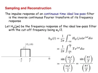
Reconstruction filters The sinc filter, while ideal, has two drawbacks: • It has large support (slow to compute) • It introduces ringing in practice The box filter is bad because its Fourier transform is a sinc filter which includes high frequency contribution from the infinite series of other copies.
Aliasing decrease sample spacing in frequency domain increase sample spacing in spatial domain
Aliasing high-frequency details leak into lower-frequency regions
Sampling theorem • For band limited function, we can just increase the sampling rate • However, few of interesting functions in computer graphics are band limited, in particular, functions with discontinuities. • It is because the discontinuity always falls between two samples and the samples provides no information of the discontinuity.
It is blurred, but better than aliasing
Antialiasing (nonuniform sampling) • The impulse train is modified as • It turns regular aliasing into noise. But random noise is less distracting than coherent aliasing.
Antialiasing (adaptive sampling) • Take more samples only when necessary. However, in practice, it is hard to know where we need supersampling. Some heuristics could be used. • It makes a less aliased image, but may not be more efficient than simple supersampling particular for complex scenes.
Application to ray tracing • Sources of aliasing: object boundary, small objects, textures and materials • Good news: we can do sampling easily • Bad news: we can’t do prefiltering • Key insight: we can never remove all aliasing, so we develop techniques to mitigate its impact on the quality of the final image.
pbrt sampling interface • Creating good sample patterns can substantially improve a ray tracer’s efficiency, allowing it to create a high-quality image with fewer rays. • core/sampling.*, samplers/*
Sampler Sampler(int xstart, int xend, int ystart, int yend, int spp); bool GetNextSample(Sample *sample); int TotalSamples() In core/scene.cpp, while (sampler->GetNextSample(sample)) { ... }
Sample Struct Sample { Sample(SurfaceIntegrator *surf, VolumeIntegrator *vol, const Scene *scene); ... float imageX, imageY; float lensU, lensV; float time; ... }
Stratified sampling • Subdivide the sampling domain into non-overlapping regions (strata) and take a single sample from each one so that it is less likely to miss important features.
Stratified sampling completely random stratified uniform stratified jittered
Comparison of sampling methods 256 samples per pixel as reference 1 sample per pixel (no jitter)
Comparison of sampling methods 1 sample per pixel (jittered) 4 samples per pixel (jittered)
High dimension • D dimension means ND cells. • Solution: make strata separately and associate them randomly, also ensuring good distributions.
Stratified sampling void StratifiedSample1D(float *samp, int nSamples, bool jitter) { float invTot = 1.f / nSamples; for (int i = 0; i < nSamples; ++i) { float delta = jitter ? RandomFloat() : 0.5f; *samp++ = (i + delta) * invTot; } } void StratifiedSample2D(float *samp, int nx, int ny, bool jitter) { float dx = 1.f / nx, dy = 1.f / ny; for (int y = 0; y < ny; ++y) for (int x = 0; x < nx; ++x) { float jx = jitter ? RandomFloat() : 0.5f; float jy = jitter ? RandomFloat() : 0.5f; *samp++ = (x + jx) * dx; *samp++ = (y + jy) * dy; } }
Stratified sampling StratifiedSample2D(imageSamples, xPixelSamples, yPixelSamples, jitterSamples); StratifiedSample2D(lensSamples, xPixelSamples, yPixelSamples, jitterSamples); StratifiedSample1D(timeSamples, xPixelSamples*yPixelSamples, jitterSamples); for (int o=0;o<2*xPixelSamples*yPixelSamples; o+=2) { imageSamples[o] += xPos; imageSamples[o+1] += yPos; } Shuffle(lensSamples, xPixelSamples*yPixelSamples, 2); Shuffle(timeSamples, xPixelSamples*yPixelSamples, 1);
Stratified sampling bool StratifiedSampler::GetNextSample(Sample *sample) { if (samplePos == xPixelSamples*yPixelSamples) { <advance to next pixel for stratified sampling> <Generate stratified camera samples> } <fill in sample by table lookup> for (u_int i = 0; i < sample->n1D.size(); ++i) LatinHypercube(sample->oneD[i],sample->n1D[i],1); for (u_int i = 0; i < sample->n2D.size(); ++i) LatinHypercube(sample->twoD[i],sample->n2D[i],2); ++samplePos; return true; }
Latin hypercube sampling • Integrators could request an arbitrary n samples. nx1 or 1xn doesn’t give a good sampling pattern. A worst case for stratified sampling
Stratified sampling reference random stratified jittered
Stratified sampling 1 camera sample and 16 shadow samples per pixel 16 camera samples and each with 1 shadow sampleper pixel
Best candidate sampling • Stratified sampling doesn’t guarantee good sampling across pixels. • Poisson disk pattern addresses this issue. The Poisson disk pattern is a group of points with no two of them closer to each other than some specified distance. • It can be generated by dart throwing. It is time-consuming. • Best-candidate algorithm by Dan Mitchell. It generates many candidates randomly and only insert the one farthest to all previous samples. • Compute a “tilable pattern” offline.
Best candidate sampling stratified jittered best candidate It avoids holes and clusters.
Best candidate sampling stratified jittered, 1 sample/pixel best candidate, 1 sample/pixel
Best candidate sampling stratified jittered, 4 sample/pixel best candidate, 4 sample/pixel
Low discrepancy sampling • Stratified sampling could suffer when there are holes or clusters. • Discrepancy can be used to evaluate the quality of a sampling pattern. for the set of AABBs with a corner at the origin
1D discrepancy Uniform is optimal! Fortunately, for higher dimension, The low-discrepancy patterns are less uniform.