Introduction to Symmetry Analysis
360 likes | 579 Vues
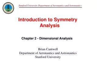
Introduction to Symmetry Analysis. Chapter 2 - Dimensional Analysis. Brian Cantwell Department of Aeronautics and Astronautics Stanford University. 2.1 Introduction. 2.2 The Two-Body Problem in a Gravitational Field. (2.1). kg. km. (2.2). Parameters of the problem. (2.3).

Introduction to Symmetry Analysis
E N D
Presentation Transcript
Introduction to Symmetry Analysis Chapter 2 - Dimensional Analysis Brian Cantwell Department of Aeronautics and Astronautics Stanford University
kg km (2.2)
Parameters of the problem (2.3) There are six parameters and three fundamental dimensions. So we can expect the solution to depend on three dimensionless numbers (2.4) and (2.5) These variables must be related by a dimensionless function of the form (2.6)
(2.7) The mean radius is defined as Theory tells us that (2.8)
2.3 The Drag on a Sphere The parameters of the problem are related to one another through a function of the form (2.9) Dimensions of the governing parameters (2.10)
The fact that the parameters have dimensions highly restricts the kind of drag functions that are possible. For example, suppose we guess that the drag law has the form (2.11a) If we introduce the dimensions of each parameter the expression has the form (2.11b) Suppose the units of mass are changed from kilograms to grams. Then the number for the drag will increase by a factor of a thousand. But the expression in parentheses will not increase by this factor and the equality will not be satisfied. In effect the drag of the sphere will seem to depend on the choice of units and this is impossible. The conclusion is that (2.11a) can not possibly describe the drag of a sphere.
The drag expression must be invariant under a three parameter dilation group. (2.12) We can derive the required drag expression as follows. Scale the units of mass using the one-parameter group (2.13) The effect is to transform the parameters as follows. (2.14) The drag expression must be independent of the scaling parameter m and therefore must be of the form. (2.15)
The dimensions of the variables remaining are (2.16) Step 2 Let the units of length be scaled according to (2.17) The effect of this group on the new variables is (2.18) The drag relation must be independent of the scaling parameter l. A functional form that accomplishes this is (2.19)
The dimensions of these variables are (2.20) Step 3 Finally scale the units of time (2.21) The effect of this group on the remaining variables is (2.22) The drag relation must be independent of the scaling parameter t. Finally (2.23) where (2.24)
In the limit of vanishing Reynolds number the drag of a sphere is given by (2.25) If we insert the expressions for the Drag coefficient and Reynolds number into Equation (2.25) the drag law becomes (2.26) Note that at low Reynolds number the drag of a sphere is independent of the density of the surrounding fluid. In this limit there is only one dimensionless parameter in the problem proportional to the product CD x Re.
One might conjecture that the same kind of law applies to the low Reynolds number flow past a circular cylinder. In this case the drag force is replaced by the drag force per unit span with units (2.27) with drag coefficient (2.28) Assume that in the limit of vanishing Reynolds number the drag coefficient of a circular cylinder follows the same law as for the sphere. (2.29) If we restore the dimensioned variables in (2.29) the result is (2.30) This is a completely incorrect result!
Measurements of circular cylinder drag versus Reynolds number taken by a variety of investigators. The data shows a huge amount of scatter - why? (2.31) The drag of a sphere or a cylinder depends on a wide variety of length and velocity scales that we have ignored!
2.4 The Drag on a Sphere in High Speed Flow The dimensions of the new variables are (2.32)
There are now two additional dimensionless variables related to the fact that the sphere motion significantly changes the temperature of the oncoming gas. (2.33) The drag relation is now a function of four dimensionless variables. (2.34) The Mach number is used in (2.34). (2.35) where (2.36) Without loss of generality we can write (2.37)
As the Mach number increases the drag coefficient tends to become independent of both Reynolds number and Mach number with (2.38)
It is important to recognize that the dimensionless parameters generated by the algorithm just described are not unique. For example in the case of the sphere we could have wound up with the following, equally correct, result. (2.41) In this form the drag law has a finite value in the limit of vanishing Reynolds number. (2.42)
R F F r Two elastic spheres pressed together Parameters Young’s modulus
Let the units of mass be scaled according to The effect of this group on the parameters is The force relation must be independent of the scaling parameter m. A functional form that accomplishes this is Note that both mass and time have been eliminated. Eliminate length
2.6 Concluding Remarks 2.7 Exercises