Download
1 / 108
1.08k likes | 1.13k Vues
Learn about Welfare Economics principles & Pareto Efficiency in evaluating policies for optimal social outcomes. Explore Pure Exchange Economy & Production Possibilities Curve concepts. Understand efficiency in resource allocation.

E N D
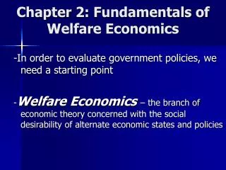
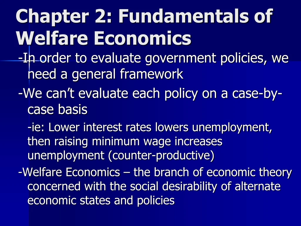
Chapter 2: Fundamentals of Welfare Economics -In order to evaluate government policies, we need a general framework -We can’t evaluate each policy on a case-by-case basis -ie: Lower interest rates lowers unemployment, then raising minimum wage increases unemployment (counter-productive) -Welfare Economics – the branch of economic theory concerned with the social desirability of alternate economic states and policies
Chapter 2: Fundamentals of Welfare Economics • Welfare Economics • First Fundamental Theorem of Welfare Economics • Second Fundamental Theorem of Welfare Economics
Starting Point: Pure Exchange Economy • We start with a simple model: • 2 people • 2 goods, each of fixed quantity • Determine good allocation • The important results of this simple, 2-person model hold in more real-world cases of many people and many commodities
Pure Exchange Economy Example • Two people: Maka and Susan • Two goods: Food (f) & Video Games (V) • We put Maka on the origin, with the y-axis representing food and the x axis representing video games • If we connect a “flipped” graph of Susan’s goods, we get an EDGEWORTH BOX, where y is all the food available and x is all the video games:
Maka’s Goods Graph Ou is Maka’s food, and Ox Is Maka’s Video Games u Food O x Video Games Maka
Edgeworth Box Susan y O’ O’w is Susan’s food, and O’y is Susan’s Video Games r Total food in the market is Or(=O’s) and total Video Games is Os (=O’r) u Food w Each point in the Edgeworth Box represents one possible good allocation O s x Video Games Maka
Edgeworth and utility • We can then add INDIFFERENCE curves to Maka’s graph (each curve indicating all combinations of goods with the same utility) • Curves farther from O have a greater utility • (For a review of indifference curves, refer to Intermediate Microeconomics) • We can then superimpose Susan’s utility curves • Curves farther from O’ have a greater utility
Maka’s Utility Curves Maka’s utility is greatest at M3 Food M3 M2 M1 O Video Games Maka
Edgeworth Box and Utility Susan O’ Susan has the highest utility at S3 r S1 A S2 At point A, Maka has utility of M3 and Susan has Utility of S2 S3 Food M3 M2 M1 O s Video Games Maka
Edgeworth Box and Utility Susan O’ If consumption is at A, Maka has utility M1 while Susan has utility S3 r A B S3 By moving to point B and then point C, Maka’s utility increases while Susan’s remains constant C Food M3 M2 M1 O s Video Games Maka
Pareto Efficiency Susan O’ Point C, where the indifference curves barely touch is called PARETO EFFICIENT, as one person can’t be made better off without harming the other. r S3 C Food M3 M2 M1 O s Video Games Maka
Pareto Efficiency • When an allocation is NOT pareto efficient, it is wasteful (at least one person could be made better off) • Pareto efficiency evaluates the desirability of an allocation • A PARETO IMPROVEMENT makes one person better off without making anyone else worth off (like the move from A to C) • However, there may be more than one pareto improvement:
Pareto Efficiency Susan O’ If we start at point A: -C is a pareto improvement that makes Maka better off -D is a pareto improvement that makes Susan better off -E is a pareto improvement that makes both better off r A S3 C S4 Food S5 E M3 M2 D M1 O s Video Games Maka
The Contract Curve • Assuming any possible starting point, we can find all possible pareto efficient points and join them to create a CONTRACT CURVE • All along the contract curve, opposing indifferent curves are TANGENT to each other • Since the slope of the indifference curve is the willingness to trade, or MARGINAL RATE OF SUBSTITUTION (x for y) (MRSxy), along this contract curve: Pareto Efficiency Condition
The Contract Curve Susan O’ r Food O s Video Games Maka
Starting Point:Economy with production • A production economy can be analyzed using the PRODUCTION POSSIBILITIES CURVE/FRONTIER • The PPC shows all combinations of 2 goods that can be produced using available inputs • The slope of the PPC shows how much of one good must be sacrificed to produce more of the other good, or MARGINAL RATE OF TRANSFORMATION (x for y) (MRTSxy) • Note that although the slope is negative, the negative is assumed and rarely shown in simple calculations
Production Possibilities Curve Here the MRTSpr is equal to (7-5)/(2-1)=-2, or two robots must be given up for an extra pizza. 10 9 8 The marginal cost of the 3rd pizza, or MCp=2 robots 7 6 The marginal cost of the 6th and 7th robots, or MCr=1 pizza Robots 5 4 Therefore, MRTSxy=MCx/MCy 3 2 Therefore, MRTSpr=2/1=2 1 1 2 3 4 5 6 7 8 Pizzas
Efficiency and Production • If production is possible in an economy, the Pareto efficiency condition becomes: • Assume that MRT>MRS. A person could transform x into y at the rate of MRS and have x left over, thus increasing his utility • Assume that MRT<MRS. A person could transform y in x at the rate of MRS and have y left over, thus increasing utility • Pareto Efficiency cannot occur at inequality
Efficiency & Production Example • Assume MRTpr=3/4 and MRSpr=2/4. • Therefore Maka could get 3 more robots by transforming 4 pizzas • BUT Maka only needs to get 2 robots for 4 pizzas to maintain utility • Therefore his utility increases from the extra robot, Pareto efficiency isn’t achieved • We can therefore reinterpret Pareto efficiency as:
First Fundamental Theorem Of Welfare Economics IF • All consumers and producers act as perfect competitors (no one has market power) and 2) A market exists for each and every commodity Then Resource allocation is Pareto Efficient
First Fundamental Theorem of Welfare Economics Origins • From microeconomic consumer theory, we know that: • Since this holds true for all people: • Which is the first requirement for Pareto efficiency, before production is considered
First Fundamental Theorem of Welfare Economics Origins • From basic economic theory, a perfect competitive firm produces where P=MC, therefore: • But we know that MRT is the ratio of MC’s, therefore:
First Fundamental Theorem of Welfare Economics Origins • Again from microeconomic consumer theory, this changes to: • But we know that MRT is the ratio of MC’s, therefore:
The Law of Demand • There is an inverse relationship between the quantity of anything that people will want to purchase and the price they must pay to obtain it: • ceteris paribus (all else held equal) • This causes demand curves to be downward sloping • When prices increase, people buy less • When prices decrease, people buy more
A B C D E The Individual’s Demand Schedule 5 4 3 Price of Songs ($) Change in Price Movement along the Demand 2 1 20 0 10 30 40 50 Number of Songs per Year
Note: We always graph P on vertical axis and Q on horizontal axis, but we write demand as Q as a function of P… If P is written as function of Q, it is called the inverse demand: Normal Form: Qd=100-2P • Inverse form: P =50 - Qd/2 • Markets defined by commodity, geography, time.
Movement Along Demand/ Changes in Quantity Demanded • A change in a good’s own price • results in a change in quantity demanded • the same thing as a movement along the same demand curve.
Shifts/Changes in Demand* • Achange inone or more of thenon-price determinantsof demand (income, tastes, etc) • results in achange indemand * • also called ashift in demand* *The whole demand schedule
Decrease in Demand Increase in Demand D2 D3 A Shift in the Demand Curve Suppose universities outlaw the use of MP3 Players Suppose the federal government gives every student a SanDisk MP3 player 5 4 3 Price of Songs ($) 2 1 D1 30 0 20 40 50 60 70 80 Quantity of Songs Demanded
“Everything Else” : The “Determinants”/ “Shifters” of “Demand” • Factors other than Price which affect “Demand” : • 1) Income, wealth • 2) Tastes and preferences • 3) The price of related goods • Complements • Substitutes • 4) Expectations • Future prices • Income • Product availability • 5) Population (market size) What movement would these factors cause?
Review of Demand Terminology • Demand: a schedule of quantities that will be bought/unit of time, at various prices, ceteris paribus. • Quantity Demanded:a specific amount that will be demanded /unit of time at a specific price, ceteris paribus. • There is a difference between between a change in the Quantity Demanded and a shift in Demand.
Price of Cigarettes, per pack Price of Cigarettes, per pack $4 $2 $2 D D’ 20 20 10 10 Number of Cigarettes smoked per day Number of Cigarettes smoked per day Shift vrs. Movement A policy to discourage smoking (no smoking in public buildings) shifts the demand curve left A tax raises the price of cigarettes, resulting in a movement along the demand curve D
Price of Kraft Dinner Price of Chicken $2 $2 D D D’ D’ 20 20 10 10 Chicken eaten in a month Kraft Dinner eaten in a month Normal vrs. Inferior Goods For normal goods, Demand decreases With income For inferior goods, Demand increases When income decrease 30
Supply: Profit • The Costside of the profitequation depends on theCosts of Productionwhich depend on • the kinds of inputs (factors of production) used • the amount of each input used • prices of inputs used • technology
Supply: Definition • A schedule that shows how much of a product a firm will supply at alternative prices for a given time period “ceteris paribus”.
The Law of Supply • The price of a product or service and the quantity supplied are directly related: “ceteris paribus” • Causes an upward sloping supply curve • The higher the price of a good, the more sellers will make available • The lower the price of a good, the fewer sellers will make available • All else being equal
F G H I Change in Price Movement along The Supply J The Individual Producer’s Supply Schedule Qnty of Songs Supplied Price / (thousands / Song year) 5 4 3 F $5 550 G 4 400 H 3 350 I 2 250 J 1 200 Price of Song ($) 2 1 0 100 200 300 400 500 600 Quantity of Songs Supplied (thousands of constant-quality units per year)
Movement Along Supply/ Changes in Quantity Supplied • A change in a good’s own price • leads to achange in quantity supplied. • that is, amovement alongthe supply curve.
Shifts/Changes in Supply • A change in one or more of the non-price determinants of supply leads to a • change in supplywhich isthe same thing asa • shift of the supply curve.
S2 S1 S2 b a b d c d A Shift in the Supply Curve When supply decreases the quantity supplied will be less at each price: ie: Singers form a union and successfully negotiate higher wages 5 When supply increases the quantity supplied will be greater at each price: ie: producer finds that she can use some cheaper singers from Newfoundland 4 3 Price of Songs ($) 2 1 40 0 20 60 80 100 120 140 Quantity of Songs Supplied (millions of constant-quality units per year)
“Everything Else” : The “Determinants”/“Shifters” of Supply • Factors other than Price that affect Supply • 1) Cost of inputs (price in factor markets) • 2) Technology and Productivity • 3) Taxes and Subsidies • 4) Price Expectations (in the product market) • 5) Number of firms in the industry How will these shift supply?
Market Equilibrium Price & Quantity • Market: where prices tend toward equality through the continuous interaction of buyers and sellers: the market forces of demand and supply Single Equilibrium Price
Putting Demand and Supply Together: Finding Market Equilibrium (1) (2) (3) (4) (5) Difference Price per Quantity Supplied Quantity Demanded (2) - (3) Constant-Quality (Songs (Songs (Songs Song per year) per year) per year) Condition $5 100 million 20 million 80 million 480 million 40 million 40 million 3 60 million 60 million 0 2 40 million 80 million -40 million 1 20 million 100 million -80 million Excess quantity supplied (surplus) Excess quantity supplied (surplus) Excess quantity demanded (shortage) Excess quantity demanded (shortage)
Excess quantity supplied at price $5 S Market clearing, or equilibrium, price E A B D Excess quantity demanded at price $1 Market Equilibrium: Definition The condition in a market when quantity supplied equals quantity demanded at a particular price; a point from where there tends to be no movement 5 4 QD= QS 3 Price pef Song ($) 2 1 0 20 40 60 80 100 Quantity of Songs (millions of constant-quality units per year)
The Law of Supply & Demand • The price of any good will adjust until the price is such that the quantity demanded is equal to the quantity supplied • A high price will result in excess supply, pushing price down, and a low price will result in excess demand, pushing price up • the market clears resulting in a single market clearing or equilibrium price.
Example: The Market for Cranberries Qd = 500 – 4p QS = -100 + 2p p = price of cranberries (dollars per barrel) Q = demand or supply in millions of barrels per year
a. The equilibrium price of cranberries is calculated by equating demand to supply: • Qd = QS … or… • 500 – 4p = -100 + 2p • …solving, • 500+100=2p+4p • p* = $100 • plug equilibrium price into either demand or supply to get equilibrium quantity: • Qd= 500-4d • Qd= 500-4(100) • Qd= 100
Example: The Market For Cranberries Price Price 125 Market Supply: P = 50 + QS/2 Market Supply: P = 50 + QS/2 P*=100 50 Market Demand: P = 125 - Qd/4 Quantity Quantity
Example: The Market For Cranberries Price 125 Market Supply: P = 50 + QS/2 • P*=100 50 Market Demand: P = 125 - Qd/4 Q* = 100 Quantity
Comparative Statics: Shifts in Demand &/or Supply • Suppose something in the demand &/or the supply “ceteris paribus” assumptions changes. • How is the MARKET affected? • 1.) Decide whether Demand &/or Supply is affected. • 2.) Decide in which direction the affected Demand &/or Supply will move. • 3.) Use a Demand and Supply diagram to determine the new equilibrium. • 4.) Calculate the new equilibrium (if possible)