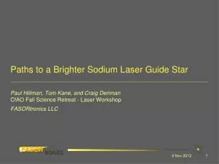
Paths to a Brighter Sodium Laser Guide Star
240 likes | 518 Vues
Paths to a Brighter Sodium Laser Guide Star. Paul Hillman, Tom Kane, and Craig Denman CfAO Fall Science Retreat - Laser Workshop FASORtronics LLC. Outline. Review Laser Guide Star Brightness History of LGSPulsed Computer Code Sodium atom energy levels/states

Paths to a Brighter Sodium Laser Guide Star
E N D
Presentation Transcript
Paths to a Brighter Sodium Laser Guide Star • Paul Hillman, Tom Kane, and Craig Denman • CfAO Fall Science Retreat - Laser Workshop • FASORtronics LLC
Outline • Review Laser Guide Star Brightness • History of LGSPulsed Computer Code • Sodium atom energy levels/states • Brightness increase method 1: Repumping • Na Doppler velocity distribution in mesosphere • Brightness increase method 2: Linewidth broadening • Atomic Recoil • Brightness increase method 3: Chirp • Atomic precession in geomagnetic field • Brightness increase method 4: Resonant pulsing at Larmor frequency • Results, comparison to CW • Frequency of short pulses to eliminate spot elongation • Possible Laser Design • Conclusion
LGSPulsed Computer Code History • Atomic Density Matrix (Simon Rochester, Dmitry Budker, UC Berkeley) • a package for Mathematica that facilitates analytic and numerical density-matrix calculations in atomic and related systems • LGSBloch (Simon Rochester, Rochester Scientific, Ron Holzlöhner, ESO) • A Mathematica package which is an extension to the Atomic Density Matrix package that contains routines for calculating the return flux from optically excited alkali atoms, specifically designed for Na atoms in the mesosphere. Mostly CW beams as it computes the steady state solution to atomic states for each velocity class. • LGSPulsed (Simon Rochester, Rochester Scientific) • A subset of LGSBloch in C to deal mostly with dynamics of pulsed beams.
F ' = = Δ ν M ' = - 3 - 2 - 1 0 1 2 3 F 4 2 . 4 M H z 3 2 P 3 / 2 - 1 5 . 9 M H z 2 - 5 0 . 3 M H z 1 0 - 6 6 . 1 M H z 3 p D 2 a 2 P = 5 8 9 . 1 5 9 0 5 n m 1 / 2 λ D 1 D 2 D 2 b = λ = 5 8 9 . 1 5 7 0 9 n m λ 5 8 9 . 1 5 8 3 3 n m = F = Δ ν 2 6 6 4 . 4 M H z 3 s 2 S 1 / 2 1 - 1 1 0 7 . 3 M H z N a D H y p e r f i n e N a D F i n e “Bohr” 2 M o d e l S t r u c t u r e S t r u c t u r e Sodium D2 Transitions • Using circular polarization, ∆mF = 1 for each absorption. • ∆mF = 1, 0, -1 for each spontaneous emission. • Driven to mF = 2 in the ground state, atoms become optically trapped and the • F=2, mF=2⬌F’=3, mF’=2 • transition dominates. • All 8 ground state levels equally populated at thermal equilibrium as: • ∆E < KT. • Method 1: pump atoms out of lower ground state.
Method 1: increasing the repump ratio • Promotes atoms out of the lower ground so they don’t accumulate there. • Assumed D2b intensity obtained by phase modulation at 1.72 GHz, there is a second sideband of equal power that does not interact with sodium. • Over a 3x improvement over no repump. • fraction power at D2b slightly dependent intensity. Intensity 47 W/m2 Linewidth: 9 MHz B = 0.5 g and 90° to beam in this and all following examples unless noted
Maxwell Boltzmann Velocity Distribution • Natural linewidth of Na is 10 MHz. • Doppler broadened linewidth is about 1 GHz or 100 velocity groups. • Method 2: As atoms become saturated at higher intensities, widening the linewidth of the laser lowers the spectral intensity and excites other nearby velocity classes.
Method 2: Increasing the Linewidth • As intensity increases optimum linewidth increases (until linewidth approaches Doppler width). • Without Repump return actually decreases with increasing linewidth! • Intensity: 500 W/m2 • D2b fraction: 14% • 40% improvement over 0 MHz
Atomic Recoil • Each absorption and emission cycle causes a 50 kHz velocity shift. • After many cycles atoms move to a higher velocity class and are not as strongly resonant with laser wavelength. • Method 3: Chirp the laser so its wavelength follows the velocity group with the highest population.
Method 3: Chirp Demonstration • Average Return: ψ = 592 ph/atom/sr/sec/(W/m2)*. • No chirp Return: ψ = 330 ph/atom/sr/sec /(W/m2)*. • Chirp rate dependent on Intensity. • Less effective for broad linewidths. • *B = 0 G, so ψ is higher in these examples. total ground states Velocity Group Population (a.u.) total excited states Doppler Shift (MHz) or Velocity Group Intensity: 47 W/m2 Chirp Rate: 0.75 MHz/µs Linewidth: 0 MHz Repump ratio: 10%
Atomic Precession • The optically pumped Na atom has a dipole cross section that is shaped like a peanut, maximized along the beam axis. • The atoms precess around magnetic field. • Precession causes the long axis of the ‘peanut’ to misalign from the beam. • The Larmor Precession frequency, fL, is proportional to the B field; at B= 0.5 G, fL = 350 kHz, or τ = 2.8 µs.
Decreased Return When Beam is not Parallel with B • As previously theorized and shown in sky tests, return flux decreases as the angle between the beam and geomagnetic field approaches 90°. CW beam LineWidth = 9 MHz Repump = 15% B field = 0.5 Gauss Intensity for CW beam = 47 W/m2
Method 4: SOLUTION, Pulse Resonantly at Larmor • Use a pulsed beam with a frequency equal to the Larmor frequency, fL. • Atom is only pumped when its highest cross section is aligned with the beam. • To our knowledge this has not been proposed before. • Note: Just amplitude modulating a CW beam is not beneficial, as ~90% of your light would be lost. An appropriate pulsed laser is necessary.
Decreased Return When Beam is not Parallel with B • Return from pulsed beam 80% greater for angles > 60° for same average power. • Pulse frequency does not depend on Intensity. Pulsed at Larmor freq. LineWidth = 150 MHz Repump = 9.2% DutyCycle = 9% CW beam LineWidth = 9 MHz Repump = 15% B field = 0.5 Gauss Intensity for CW beam = 47 W/m2 Avg. Intensity = 47 W/m2, Peak Intensity for pulsed beam = 522 W/m2 Pulse Frequency = 350 kHz
What Observatories Could Benefit? • Inclination for Hawaii (H) is ~35° • For zenith propagation angle between beam and B is 55° • Inclination for Antofagasta, Chile (A) is ~ 20° • For zenith propagation angle between beam and B is 70° Geomagnetic Main Field Inclination H A NOAA/NGDC & CIRES - 2010 Green line is 0° Bold Contours are 20° intervals
Summary of Results - Pulsed at Larmor Frequency Angle between beam and B field is 90° B = 0.5 G
Summary of Results - CW Angle between beam and B field is 90° B = 0.5 G
Comparison of Efficiencies • Plotted is the mesospheric flux (ph/atom/sr/sec) divided by Intensity. • CW is slightly lower than Holzlöhner (2009) as that work only considered power going into a single side band, not two as here. Pulsed at fL CW Angle between beam and B field is 90° B = 0.5 G
Photon Flux at Telescope, 0.6 - 1 arcsec seeing LGS size similar to Holzlöhner (2009), equivalent Gaussian FWHM = 40.4 cm. Magnitude V = 4.7 for a flux of 10,000; Drummond (2004).
Extension to Single Pulse at a time in Mesosphere • Outside sub-apertures of large telescopes see an elongated spot with CW lasers. Ideally only a single short pulse in the mesosphere at a time optimum. • Technique is effective at fL / N sub-harmonics. Rep. rate needs to be < spin relaxation rate. • Wrong pulse rep. rate could result in a 40% decrease in photon return. Intensity = 3.7 W/m2 frequency = 30.4 kHz For both plots: Peak Intensity = 500 W/m2 Pulse length = 0.26 µs Linewidth = 150 MHz, Repump = 9% (Parameters were not optimized) Intensity = 3.9 W/m2 frequency = 29.2 kHz
Laser Design to Obtain Beam Pulse Format • System still based on sum frequency mixing in LBO • LBO in 1.319µ laser cavity to obtain high intensity • 1.064µ is generated by a low power laser, modulated, then amplified. It is only single pass through LBO. • High power, single spatial mode fiber amplifiers are COTS. • Since 1.064µ is not resonant in a cavity, it can have a large linewidth • Modulation is done at low power • Only one resonant cavity
Conclusions • For the 20 W average power lasers being considered for today’s sodium guide stars, a 2.2 x higher return can be obtained by pulsing mesospheric sodium resonantly at the Larmor frequency (~ 175 - 350 kHz) • Improvement is noted even at fL/10, 35 kHz or τ = 28 µs, as this is still much less than the spin relaxation rate of ~250µs. This is an ideal pulse format for large telescopes that want a pulse format to eliminate LGS elongation. • The higher return flux needed for AO in the visible is possible from sodium laser guide stars, the return flux is not limited by sodium abundance or sodium physics but by appropriate beam pulse format and laser power. • Chirping a narrow linewidth laser can increase return by over a factor of 2, but becomes less beneficial for broader linewidths.