Optimizing Protocol Design Through Context-Aware Mobility and User Behavior Analysis
This paper explores the challenges of suboptimal performance in protocol design due to a lack of understanding of user context and behavior. By leveraging extensive trace-based analysis, we identify dominant trends in individual and collective user behavior within mobile environments. We propose a framework utilizing insights from mobility modeling, behavioral grouping, and information dissemination to inform the design of future context-aware protocols. Our findings are grounded in comprehensive studies from multiple university campuses, providing a rich dataset to enhance future wireless network evaluations.

Optimizing Protocol Design Through Context-Aware Mobility and User Behavior Analysis
E N D
Presentation Transcript
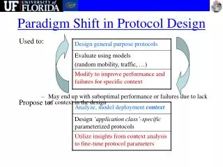
Paradigm Shift in Protocol Design Used to: • May end up with suboptimal performance or failures due to lack of context in the design Propose to:
Problem Statement • How to gain insight into deployment context? • How to utilize insight to design future services? Approach • Extensive trace-based analysis to identify dominant trends & characteristics • Analyze user behavioral patterns • Individual user behavior and mobility • Collective user behavior: grouping, encounters • Integrate findings in modeling and protocol design • I. User mobility modeling – II. Behavioral grouping • III. Information dissemination in mobile societies, profile-cast
Analyze Represent Trace Characterize (Cluster) The TRACE framework MobiLib Employ (Modeling & Protocol Design)
Trace Vision:Community-wide Wireless/Mobility Library • Library of • Measurements from Universities, vehicular networks • Realistic models of behavior (mobility, traffic, friendship, encounters) • Benchmarks for simulation and evaluation • Tools for trace data mining • Use insights to design future context-aware protocols? • http://nile.cise.ufl.edu/MobiLib
Trace Libraries of Wireless Traces • Multi-campus (community-wide) traces: • MobiLib (USC (04-06), now @ UFL) • nile.cise.ufl.edu/MobiLib • 15+ Traces from: USC, Dartmouth, MIT, UCSD, UCSB, UNC, UMass, GATech, Cambridge, UFL, … • Tools for mobility modeling (IMPORTANT, TVC), data mining • CRAWDAD (Dartmouth) • Types of traces: • University Campus (mainly WLANs) • Conference AP and encounter traces • Municipal (off-campus) wireless • Bus & vehicular wireless networks • Others … (on going)
Trace Wireless Networks and Mobility Measurements • In our case studies we use WLAN traces • From University campuses & corporate networks (4 universities, 1 corporate network) • The largest data sets about wireless network users available to date (# users / lengths) • No bias: not “special-purpose”, data from all users in the network • We also analyze • Vehicular movement trace (Cab-spotting) • Human encounter trace (at Infocom Conf)
Case Study I: Goal • To understand the mobility/usage pattern of individual wireless network users • To observe how environments/user type/trace-collection techniques impact the observations • To propose a realistic mobility model based on empirical observations • That is mathematically tractable • That is capable of characterizing multiple classes of mobility scenarios
IMPACT: Investigation of Mobile-user Patterns Across University Campuses using WLAN Trace Analysis* - 4 major campuses – 30 day traces studied from 2+ years of traces - Total users > 12,000 users - Total Access Points > 1,300 • Understand changes of user association behavior w.r.t. • Time - Environment - Device type - Trace collection method * W. Hsu, A. Helmy, “IMPACT: Investigation of Mobile-user Patterns Across University Campuses using WLAN Trace Analysis”, two papers at IEEE Wireless Networks Measurements (WiNMee), April 2006
Represent Metrics for Individual Mobility Analysis • What kind of spatial preference do users exhibit? • The percentile of time spent at the most frequently visited locations • What kind of temporal repetition do users exhibit? • The probability of re-appearance • How often are the nodes present? • Percentage of “online” time
Observations: Visited Access Points (APs) Fraction of online time associated with the AP Prob.(coverage > x) CCDF of coverage of users [percentage of visited APs] Average fraction of time a MN associates with APs • Individual users access only a very small portion of APs in the network. • On average a user spends more than 95% of time at its top 5 most visited APs. • Long-term mobility is highly skewed in terms of time associated with each AP. • Users exhibit “on”/”off” behavior that needs to be modeled.
Repetitive Behavior • Clear repetitive patterns of association in wireless network users. • Typically, user association patterns show the strongest repetitive pattern at time gap of one day/one week.
Skewed location preference Characterize On/off activity pattern Periodic re-appearance Prob.(online time fraction > x) Mobility Characteristics from WLANs • Simple existing modelsare very differentfrom the characteristicsin WLAN
Mobility Models • Mobility models are of crucial importance for the evaluation of wireless mobile networks [IMP03] • Requirements for mobility models • Realism (detailed behavior from traces) • Parameterized, tunable behavior • Mathematical tractability • Related work on mobility modeling • Random models (Random walk/waypoint): inadequate for human mobility • Improved synthetic models (pathway model, RPGM, WWP, FWY, MH) – more realistic, difficult to analyze • Trace-based model (T/T++): trace-specific, not general
75% 25% Employ Time-variant Community (TVC) Model(W. Hsu, Thyro, K. Psounis, A. Helmy, “Modeling Time-variant User Mobility in Wireless Mobile Networks”, IEEE INFOCOM, 2007, Trans. on Networking 2009) • Skewed location visiting preference • Create “communities” to be the preferred area of movement • Each node can have its own community • Node moves with two different epoch types – Local or roaming • Each epoch is a random-direction,straight-line movement • Local epochs in the community • Roaming epochs around the whole simulation area
Employ Tiered Time-variant Community (TVC) Model • Periodical re-appearance • Create structure in time – Periods • Node moves with different parameters in periods to capture time-dependent mobility • Repetitive structure • Finer granularity in space & time • Multi-tier communities • Multiple time periods
Using the TVC Model – Reproducing Mobility Characteristics • (STEP1) Identify the popular locations; assign communities • (STEP2) Assignparameters to the communities according to stats • (STEP3) Add user on-off patterns (e.g., in WLAN, users are usually off when moving)
Using the TVC Model – Reproducing Mobility Characteristics • WLAN trace (example: MIT trace) Skewed location visiting preference Periodic re-appearance * Model-simplified: single community per node. Model-complex: multiple communities ** Similar matches achieved for USC and Dartmouth traces
Using the TVC Model – Reproducing Mobility Characteristics • Vehicular trace (Cab-spotting)
Using the TVC Model – Reproducing Mobility Characteristics • Human encounter trace at a conference Inter-meeting time A encounters B Encounter duration time Encounter duration Inter-meeting time
Case Study II: Goal • Identify similar users (in terms of long run mobility preferences) from the diverse WLAN user population • Understand the constituents of the population • Identify potential groups for group-aware service • In this case study we classify users based on their mobility trends (or location-visiting preferences) • We consider semester-long USC trace (spring 2006, 94days) and quarter-long Dartmouth trace (spring 2004, 61 days)
Association vector: (library, office, class) =(0.2, 0.4, 0.4) Represent Representation of User Association Patterns • We choose to represent summary of user association in each day by a single vector • a = {aj : fraction of online time user i spends at APj on day d} • Summarize the long-run mobility in an “association matrix” • Office, 10AM -12PM • Library, 3PM – 4PM-Class, 6PM – 8PM
Eigen-behavior • Eigen-behaviors: The vectors that describe the maximum remaining power in the association matrix (obtained through Singular Value Decompostion)with quantifiable importance • Eigen-behavior Distance calculates similarity of users by weighted inner products of eigen-behaviors. • Assoc. patterns can be re-constructed with low rank & error • Benefits: Reduced computation and noise
Similarity-based User Classification • With the distance between users U and V defined as 1-Sim(U,V), we use hierarchical clustering to find similar user groups. USC Dartmouth *AMVD = Average Minimum Vector Distance
Validation of User Groups • Significance of the groups – users in the same group are indeed much more similar to each other than randomly formed groups (0.93 v.s. 0.46 for USC, 0.91 v.s. 0.42 for Dartmouth) • Uniqueness of the groups – the most important group eigen-behavior is important for its own group but not other groups
User Groups in WLAN - Observations • Identified hundreds of distinct groups of similar users • Skewed group size distribution – the largest 10 groups account for more than 30% of population on campus. Power-law distributed group sizes. • Most groups can be described by a list of locations with a clear ordering of importance • We also observe groups visiting multiple locations with similar importance – taking the most important location for each user is not sufficient
Case Study III: Goal • Understand inter-node encounter patterns from a global perspective • How do we represent encounter patterns? • How do the encounter patterns influence network connectivity and communication protocols? • Encounter definition: • In WLAN: When two mobile nodes access the same AP at the same timethey have an‘encounter’ • In DTN: When two mobile nodes move within communication range they have an‘encounter’
Observations: Encounters Prob. (unique encounter fraction > x) Prob. (total encounter events > x) CCDF of unique encounter count CCDF of total encounter count • In all the traces, the MNs encounter a small fraction of the user population. • A user encounters 1.8%-6% on averageof the user population (except UCSD) • The number of total encounters for the users follows a BiPareto distribution.
Group of good friends… Cliques with random links to join them Represent Encounter-Relationship (ER) graph • Draw a link to connect a pair of nodes if they ever encounter with each other … Analyze the graph properties?
Small World Small Worlds of Encounters • Encounter graph: nodes as vertices and edges link all vertices that encounter Regular graph Clustering Coefficient (CC) Normalized CC and PL Av. Path Length Random graph • The encounter graph is a Small World graph (high CC, low PL) • Even for short time period (1 day) its metrics (CC, PL) almost saturate
B A C Background: Delay Tolerant Networks (DTN) • DTNs are mobile networks with sparse, intermittent nodal connectivity • Encounter events provide the communication opportunities among nodes • Messages are stored and moved across the network with nodal mobility
Trace duration = 15 days (Fig: USC) Unreachable ratio Information Diffusion in DTNs via Encounters • Epidemic routing (spatio-temporal broadcast) achieves almost complete delivery Robust to the removal of short encounters Robust to selfish nodes (up to ~40%)
Encounter-graphs using Friends • Distribution for friendship index FI is exponential for all the traces • Friendship between MNs is highly asymmetric • Among all node pairs: < 5% with FI > 0.01, and <1% with FI > 0.4 • Top-ranked friends form cliques and low-ranked friends are key to provide random links (short cuts) to reduce the degree of separation in encounter graph.
Is B similar to V? Is E similar to V? ? Is C/D similar to V? Profile-castW. Hsu, D. Dutta, A. Helmy, ACM Mobicom 2007 • Sending messages to others with similar behavior, without knowing their identity • Announcements to users with specific behavior V • Interest-based ads, similarity resource discovery • Assuming DTN-like environment C B E D A
Profile-cast Use Cases • Mobility-based profile-cast • Targeting group of users who move in a particular pattern (lost-and-found, context-aware messages, moviegoers) • Approach: use “similarity metric” between users • Mobility-independent profile-cast • Targeting people with a certain characteristics independent of mobility (classic music lovers) • Approach: use “Small World” encounter patterns
Mobility space S N D N N N S D D Forward?? Mobility-based Profile-cast Scoped message spread in the mobility space
1. profiling S N N N N Each row represents an association vector for a time slot An entry represents the percentage of online time during time slot i at location j Sum. vectors Profile-cast Operation • Profiling user mobility • The mobility of a node is represented by an association matrix • Singular value decomposition provides a summary of the matrix (A few eigen-behavior vectors are sufficient, e.g. for 99% of users at most 7 vectors describe 90% of power in the association matrix)
1. profiling S N N N N 2. Forwarding decision Profile-cast Operation • Determining user similarity • S sends Eigen behaviors for the virtual profile to N • N evaluated the similarity by weighted inner products of Eigen-behaviors • Message forwarded if Sim(U,V) is high (the goal is to deliver messages to nodes with similar profile) • Privacy conserving: N and S do not send information about their own behavior
* Results presented as the ratio to epidemic routing Profile-cast Evaluation • Epidemic: Near perfect delivery ratio, low delay, high overhead • Centralized: Near perfect delivery ratio, low overhead, a bit extra delay • Decentral: provides tradeoff between delivery & overhead • Random: poor delivery ratio Epidemic Decentral Decentral Decentral Random Random Random Random - Decentralized I-cast achieves: > 50% reduction in overhead of Epidemic >30% increase in delivery of Random
Success Rate Delay Overhead 92% 45% more overhead Evaluation - Result • Centralized: Excellent successrate with only 3% overhead. • Similarity-based: • (1) 61% success rate at low overhead, 92% success rate at 45% overhead • (2) A flexible success rate – overhead tradeoff • RTx with infinite TTL: Much more overhead undersimilar success rate • Short RTx with many copies: Good success rate/overhead, but delay is still long
Flooding Flood-sim S S S S S Single long random walk Multiple short random walks Mobility Profile-cast (intra-group) Goal
S S S S S S T.P. T.P. T.P. T.P. T.P. T.P. Gradient-ascend Single long random walk Multiple short random walks Mobility Profile-cast (inter-group) Goal Flooding Flooding_sim
Performance Comparison Gradient ascend helpsto overcome the difficult case – when the source is far from T.P. Few long RW is better when S is far from T.P. but many short RW is betterwhen S is close to T.P.
Performance Comparison Few long RW is better when S is close toT.P. but many short RW is betterwhen S is close to T.P. Gradient ascend helpsto overcome the difficult case – when the source is far from T.P. Gradient ascend has some extra delay compared with flooding
Profile-cast Initial Results • Adjustable overhead/delivery rate tradeoff • 61% delivery rate of flooding with 3% overhead • 92% delivery rate with 45% overhead • Better than single random walk in terms of delay, delivery rate • Multiple short random walks also work well in this case
S S S S S Mobility Independent Profile-cast Goal Flooding SmallWorld-based Single long random walk Multiple short random walks
Future Work • Sending to a mobility profile specified by the sender • Gradient ascend followed by similarity comparison (in the mobility space) • Mobility independent profile-cast • The encounter pattern provides a network in which most nodes are reachable • We don’t want to flood – How to leverage the Small World encounter pattern to reach the “neighborhood” of most nodes efficiently?
Future Work • One-copy-per-clique in the “mobility space” • We expect this to work because similarity in mobility leads to frequent encounters