Comprehensive Guide to Assumption Checking in Stata Regression Analysis
This manual serves as a detailed resource for checking assumptions in regression and logistic regression analysis using Stata. It covers essential topics including multi-collinearity, homoscedasticity, linearity, and the normal distribution of errors. The guide provides practical Stata commands to detect issues, addresses common pitfalls, and offers solutions such as multi-level analyses and utilizing user-created commands. With clear explanations and examples, this document aims to simplify the regression analysis process for users transitioning from SPSS to Stata.

Comprehensive Guide to Assumption Checking in Stata Regression Analysis
E N D
Presentation Transcript
Stata manuals You have all these as pdf! Check the folder /Stata12/docs
ASSUMPTION CHECKING AND OTHER NUISANCES • In regression analysis with Stata • In logistic regression analysis with Stata NOTE: THIS WILL BE EASIER IN Stata THAN IT WAS IN SPSS
Assumption checking in “normal” multiple regression with Stata
Assumptions in regression analysis • No multi-collinearity • All relevant predictor variables • included • Homoscedasticity: all residuals are • from a distribution with the same variance • Linearity: the “true” model should be • linear. • Independent errors: having information • about the value of a residual should not • give you information about the value of • other residuals • Errors are distributed normally
FIRST THE ONE THAT LEADS TO NOTHING NEW IN STATA (NOTE: SLIDE TAKEN LITERALLY FROM MMBR) Independent errors: havinginformationabout the value of a residualshouldnotgiveyouinformationabout the value of otherresiduals Detect: askyourselfwhetherit is likelythatknowledgeaboutoneresidualwouldtellyousomethingabout the value of anotherresidual. Typical cases: -repeatedmeasures -clusteredobservations (peoplewithinfirms / pupilswithin schools) Consequences: as forheteroscedasticity Usually, yourconfidenceintervals are estimatedtoosmall (thinkaboutwhythat is!). Cure: usemulti-level analyses part 2 of this course
The rest, in Stata: Example: the Stata “auto.dta” data set sysuse auto corr (correlation) vif (variance inflation factors) ovtest (omitted variable test) hettest (heterogeneity test) predict e, resid swilk (test for normality)
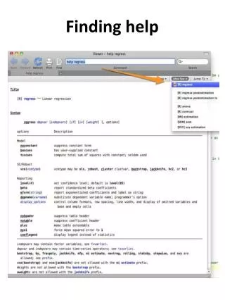
Finding the commands • “help regress” • “regress postestimation” and you will find most of them (and more) there
Multi-collinearity A strongcorrelationbetweentwoor more of your predictor variables Youdon’t want it, because: • It is more difficult to gethigher R’s • The importance of predictorscanbedifficult to establish (b-hatstend to go to zero) • The estimatesforb-hats are unstableunderslightly different regressionattempts (“bouncingbeta’s”) Detect: • Look at correlation matrix of predictor variables • calculateVIF-factorswhile running regression Cure: Delete variables sothatmulti-collinearitydisappears, forinstancebycombiningtheminto a single variable
Stata: calculating the correlation matrix (“corr” or “pwcorr”) and VIF statistics (“vif”)
Misspecification tests(replaces: all relevant predictor variables included) Also run “ovtest, rhs” here. Both tests should be non-significant. Note that there are two ways to interpret “all relevant predictor variables included”
Homoscedasticity: all residuals are from a distribution with the samevariance This can be done in Stata too (check for yourself) Consequences: Heteroscedasticiy does notnecessarilylead to biases in yourestimatedcoefficients (b-hat), butit does lead to biases in the estimate of the width of the confidence interval, and the estimation procedure itself is notefficient.
Testing for heteroscedasticity in Stata • Your residuals should have the same variance for all values of Y hettest • Your residuals should have the same variance for all values of X hettest, rhs
Errorsdistributednormally Errorsshouldbedistributednormally (justthe errors, not the variables themselves!) Detect: look at the residual plots, test fornormality, or save residualsand test directly Consequences: rule of thumb: ifn>600, noproblem. Otherwiseconfidenceintervals are wrong. Cure: try to fit a bettermodel (or use more difficultways of modelinginstead- askan expert).
Errorsdistributednormally First calculate the errors (after regress): predict e, resid Then test for normality swilke
Assumption checking in logistic regression with Stata Note: based on http://www.ats.ucla.edu/stat/stata/webbooks/logistic/chapter3/statalog3.htm
Assumptions in logistic regression • Y is 0/1 • Independence of errors (as in multiple regression) • No cases where you have complete separation (Stata will try to remove these cases automatically) • Linearity in the logit (comparable to “the true model should be linear” in multiple regression) – “specification error” • No multi-collinearity (as in m.r.) Think!
Think! • What will happen if you try logit y x1 x2 in this case?
This! Because all cases with x==1 lead to y==1, the weight of x should be +infinity. Stata therefore rightly disregards these cases. Do realize that, even though you do not see them in the regression, these are extremely important cases!
(checking for)multi-collinearity • In regression, we had “vif” • Here we need to download a command that a user-created: “collin” (try “finditcollin” in Stata)
(checking for)specification error • The equivalent for “ovtest” is the command “linktest”
Further things to do: • Check for useful transformations of variables, and interaction effects • Check for outliers / influential cases: 1) using a plot of stdres (against n) and dbeta(against n) 2) using a plot of ldfbeta’s(against n) 3) using regress and diag (but don’t tell anyone that I suggested this)
Checking for outliers … check the file auto_outliers.do for this …