Understanding High Ozone Levels in Winter: Influence of Snow Cover and Terrain Features
Explore the factors contributing to elevated winter ozone concentrations, such as stable layers trapping NOx and VOCs, impact of snow cover on ozone near the surface, and terrain effects. Analyze data from various simulations and observations to assess ozone variability.

Understanding High Ozone Levels in Winter: Influence of Snow Cover and Terrain Features
E N D
Presentation Transcript
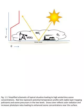
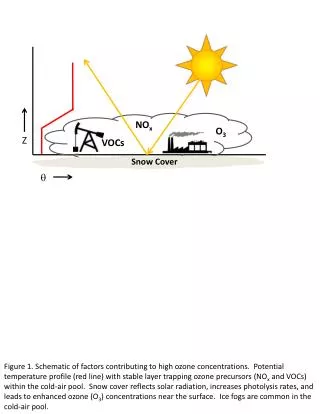
NOx VOCs O3 Snow Cover Z q Figure 1. Schematic of factors contributing to high ozone concentrations. Potential temperature profile (red line) with stable layer trapping ozone precursors (NOx and VOCs) within the cold-air pool. Snow cover reflects solar radiation, increases photolysis rates, and leads to enhanced ozone (O3) concentrations near the surface. Ice fogs are common in the cold-air pool.
4500 (a) 4000 3500 3000 2500 2000 1.33 km 4 km 1500 1000 500 12 km 0 4000 WY (b) 3750 3500 Uinta Mountains UT CO 3250 3000 VER ROO 2750 Wasatch Range RED 2500 MYT HOR OUR 2250 Tavaputs 2000 1750 Plateau 1500 Desolation Canyon 1250 Figure 2. (a) WRF 12-, 4-, and 1.33-km domains with terrain contoured every 500 m. (b) Uintah Basin subdomain with terrain contoured every 250 m and major geographic features labeled. Black dots indicate locations of surface stations used for verification: Horsepool (HOR), Myton (MYT), Ouray (OUR), Red Wash (RED), Roosevelt (ROO), and Vernal (VER). Red line indicates position of vertical cross sections shown later.
Figure 3. Snow depth (blue) and snow water equivalent (red) as a function of elevation for 0000 UTC 1 February 2013 for: prescribed snow applied to WRF simulations (black line); observations (O) from the Uintah Basin and surrounding mountains; and NAM analysis (X). NAM analysis data were extracted along a southeast to northwest transect from the center of the basin to the center of the Uinta Mountains.
(b) (a) (d) (c) Figure 4. WRF surface albedo (top) at 0100 UTC 1 February 2013 for (a) before and (b) after modifications to WRF snow albedo and vegetation parameter table. Initialized snow depth (bottom, in m) at 0000 UTC 1 February 2013 for (a) “Full Snow” cases (BASE/FULL) and (b) “No Snow” case (NONE). Terrain contoured every 500 m in black.
(a) (b) Figure 5. SPoRT-derived VIIRS satellite images: (a) Snow-Cloud product at 1815 UTC 2 February 2013 and (b) Nighttime Microphysics RGB product at 0931 UTC 2 February 2013.
(b) (a) (c) (d) (e) (f) (g) (h) Figure 6. Observed and simulated vertical profiles at Roosevelt of (a, b) potential temperature, (c, d) relative humidity with respect to ice, (e, f) wind speed, and (g, h) wind direction for 1800 UTC 4 February 2013 (left) and 1800 UTC 5 February 2013 (right).
(a) 4 km (b) Day of February Figure 7. (a) Hourly ozone concentrations from 1-6 February 2013 for Roosevelt (black), Horsepool (blue), Vernal (red), and Ouray (green) with the 75 ppb (8-hour mean) NAAQS denoted by the dashed line. (b) Ceilometer backscatter (shaded) and estimated aerosol depth (black dots) as a function of height (m) at Roosevelt from 1-7 February 2013. Red, yellow, blue, and white shading denote fog and stratus clouds, high aerosol concentrations; low aerosol concentrations, and beam attenuation, respectively.
(a) (b) (c) -2 0 -8 -12 -10 -6 -4 2 Figure 8. Average 2-m temperature (in °C according to the scale below) for 1–6 February 2013 from (a) BASE, (b) FULL, and (c) NONE simulations.
(a) 20 15 10 5 0 2 (b) 1.5 1 0.5 0 -0.5 -5 Figure 9. Average difference (BASE – FULL) for 1–6 February 2013 period in: (a) 2-m temperature (in °C according to the scale to the right) and (b) downwelling longwave radiation (in W m-2 according to the scale on the right)
300 2.6 (a) BASE 298 2.4 2.2 296 Height (km) 2.0 294 1.8 292 1.6 290 2.6 (b) FULL 288 2.4 286 2.2 Height (km) 2.0 284 1.8 282 1.6 280 2.6 (c) NONE 278 2.4 276 2.2 Height (km) 274 2.0 2 7 4 3 1 5 6 272 1.8 1.6 270 Day of February Figure 10. Time-height plot of potential temperature (in K according to the scale on the right) at Horsepool from 1–6 February 2013 from (a) BASE, (b) FULL, and (c) NONE simulations.
0.25 0.25 (a) (b) 0.2 0.2 0.15 0.15 0.1 0.1 0.05 0.05 0 0 0.30 0.30 (c) (d) 0.20 0.20 0.1 0.1 0 0 (f) (e) 120 120 100 100 80 80 60 60 40 40 20 20 0 0 Figure 11. Cloud characteristics from BASE (a, c, e) and FULL (b, d, f) simulations at 0600 UTC 5 February 2013. (a, b) Integrated cloud amount (in mm according to the scale on the right), (c) mean cloud water in bottom 15 model levels (in g kg-1 according to the scale on the right), (d) mean cloud ice in bottom 15 model levels (in g kg-1 according to the scale on the right), (e, f) net downwelling longwave radiation from clouds (in W m-2 according to the scale on the right).
(a) 40 35 30 25 20 15 10 5 0 STA ROO OUR HOR 3.0 (b) 304 302 300 298 2.5 296 294 292 Height (km) 290 288 2.0 286 284 282 280 278 1.5 276 50 200 100 150 W E Distance (km) Figure 12. FULL simulation at 0600 UTC 4 February 2013 for (a) 2.3 km MSL wind speed (in m s-1 according to the scale on the right) and barbs (full barb 5 m s-1). (b) Vertical cross section of potential temperature (in K according to the scale on the right) along red line in (a).
5 3.0 (b) (a) 2.8 4 2.6 2.4 3 Height (km) 2.2 2.0 2 1.8 1 1.6 1.4 0 3.0 (d) (c) 2.8 -1 2.6 -2 2.4 2.2 Height (km) -3 2.0 1.8 -4 1.6 -5 1.4 Figure 13. Average zonal wind in the vicinity of the cross-section in Fig. 2b for the 1-6 February 2013 period. The FULL simulation (top) and NONE simulation (bottom) results for (a, c) daytime hours (0800 to 1700 MST) and (b, d) nighttime hours (1800 to 0700 MST). Westerly (easterly) winds shaded in m s-1 according to the scale on the right in red (blue) with westerly (easterly) winds contoured every 2 m s-1 ( -0.5, -1, and -2 m s-1 only). Values are averaged over a 26-km wide swath perpendicular to the cross section.
(a) Vernal Roosevelt Duchesne River Green River Ouray White River (b) Figure 14. Mobile transect of ozone concentration from 1130 to 1500 MST 6 February 2013 as a function of (a) geographic location and (b) time. Dashed black line represents NAAQS for ozone (75 ppb).
100 (a) (b) 90 80 70 3.0 3.0 (c) (d) 60 2.8 2.8 2.6 2.6 2.4 2.4 50 2.2 2.2 Height (km) Height (km) 2.0 2.0 1.8 1.8 40 1.6 1.6 1.4 1.4 1.2 1.2 30 Figure 15. (top)Average ozone concentration (in ppb according to scale on the right) during 1100-1700 MST 1–6 February 2013 on the lowest CMAQ model level (~17.5 m) from (a) FULL and (b) NONE simulations. The thin black line outlines regions where the ozone concentration exceeds 75 ppb while the reference terrain elevation of 1800 m is shown by the heavy black line. (bottom) Average ozone concentration during 1100-1700 MST 1–6 February 2013 from (c) FULL and (d) NONE simulations along cross section approximately 25 km south of the red line in Fig. 2b. Values averaged over 24-km wide swath perpendicular to the cross section.
(a) (b) 300 2.6 (c) 295 2.4 290 2.2 285 Height (km) 2.0 280 1.8 275 1.6 270 Figure 16. Time Series of ozone concentrations from (a) Roosevelt, and (b) Horsepool. Observations, CMAQ output from FULL and NONE simulations in blue, red, and black respectively. The NAAQS of 75 ppb is denoted by the thin black dashed line. (c) Time-Height of potential temperature (shaded according to scale on right and contoured in thin black) and ozone concentrations at Horsepool from FULL simulation. Ozone concentrations are contoured every 10 ppb, starting at 75 ppb and alternate between solid and dashed every 10 ppb. Plotted ozone concentrations represent the maximum value for each hour in a 40 by 40 km region encompassing Ouray and Horsepool .
Table 3. 2-m temperature errors from WRF simulations. Mean errors calculated from the six surface stations in Fig. 1.5b during the 1-6 February 2013 period.
Table 4. Ozone concentration statistics from CMAQ model forced by FULL and NONE simulations during the 1-6 February 2013 period.