Oceanographic Sampling in VOCALS REx
280 likes | 398 Vues
This report summarizes oceanographic sampling conducted in the Southeast Pacific (SEP) as part of the VOCALS REx project. The region is characterized by persistent trade winds, coastal upwelling, and varying salinity layers, influencing surface temperature and ocean dynamics. Key objectives include understanding controls on sea surface temperature (SST) and exploring the oxygen minimum layer. Data from two moorings provide insights into surface fluxes, eddy variability, and the interaction between wind-driven currents and oceanographic features, highlighting the importance of local and remote forcings.

Oceanographic Sampling in VOCALS REx
E N D
Presentation Transcript
Oceanographic Samplingin VOCALS REx Bob Weller rweller@whoi.edu
The ocean setting - the Southeast Pacific (SEP) • Persistent trade winds, coastal upwelling. • Trade winds - directionally steady but vary in speed, with periods of low winds • Low level of synoptic weather systems • Peru/Chile Current flowing north and northwest.
• A strongly evaporative, moderately warmed region producing temperate, salty surface water. • Fresher water moving in below the surface layer. • Below that a more saline layer and a second salinity minimum. • Coastal upwelling. • Westward propagating eddies originating from coast. • VOCALS’ goal of understanding controls on SST sets a focus on the surface layer • VOCALS partners (Chile,Peru, France - PRIMO, SOLAS) interest is on the oxygen minimum layer below The ocean setting temperature salinity 20°S, 85°W
October-November: Deep (150 m), cool layer transitioning to warm, shallow (40 m) layer Mixed layer depths 0.1, 0.5, 1.0 delta T from SST
~1 cm/sec ~ 3 cm/sec 3 year displacement at 10 m depth, a mean of ~ 3 cm/sec 3 year displacement at 350 m depth, a mean of ~ 1 cm/sec In upper thermocline, 1-2 cm/sec annual mean Flows to NW; low rates of advection. Long residence time? Eddy variability superimposed on the mean.
1000 500 130 m 0 Distance (km) -500 10 m – 130 m -1000 20 m – 130 m -1000 Distance (km) 0 500 Steady Trade Winds to the NW, wind-driven surface flow to the Southwest One-year displacements or progressive vector diagrams of velocities at 10 and 20 m relative to that at 130 m, as well as for the velocity at 130 m. The surface water moves offshore under the influence of the wind. ~5 cm s-1 surface layer relative to thermocline.
QuikScat winds and TMI SST fields used to estimate the advective component of heat flux due to Ekman transport across SST gradients. Calculation done for weekly fields and then combined to get an annual average. The steadiness of the winds implies that the mean of the high-frequency product is close to the product of the means. Ekman Advection along SST gradients Color Contours: Annually averaged component of the heat flux due to advection by Ekman transport Gray Contours: Annually averages SST Arrows: Annually averaged Ekman transport Ekman Advection = 6 +/- 5 W/m2
Surface forcing from buoy driving a one-dimensional ocean model (PWP) produces a surface layer that is too warm and too salty. ) Weller
Additional cooling and freshening is needed. Possible mechanisms:- Ekman (wind-driven surface layer) transport offshore of coastal water- Open ocean downwelling/upwelling (Ekman pumping)- Mixing with low saline water below- Geostrophic currents (advection)- Eddy processes, including horizontal transport enhanced vertical mixing Remote as well as local forcing is possible, possible links to ENSO variability. - Kelvin waves->coastal waves-> Rossby waves - Displacement of S Pacific high pressure center Integrated Heat Content Equation Surface Flux Advection Ekman Pumping Eddy Flux Divergence Vertical Diffusivity
Altimetric satellites show westward propagating eddies are typical of the region. Propagation ~ 5 cm s-1 Size ~ 4° or 440 km Residence time ~ 100 days S-P Xie
Eddies – biology and clouds Long-lived eddies: • Transport or enhancement of nutrients • Enhanced local productivity • Change in upper ocean optical properties • Biogenic aerosols – DMS • Local SST and current signature (impacting fluxes via delta U and delta T)
Fast time scales to cope with as well Diurnal – 24 hours
A progression of daily composite wind speeds from QuikScat in 2001. The darkest blue contour represents wind speeds below 2m s-1 (contour increment is 2 m s-1).Diurnal warming linked to “sagging” of the Trade Winds.Does the whole dark blue region warm 2°C? If so,what impact on clouds?
Shallow, near-inertial oscillations Current speed at indicated depth Transients in wind lead to near-inertial oscillationsand probable shear-driven mixinglocal inertial period ~36 hours cm/s cm/sec yearday
Sampling issues • Relatively shallow ocean mixed layer, but in transition • Good vertical resolution in upper 300 m • Good temporal resolution in upper 300 m • Good surface fluxes • High stability and strong property gradients at base • Eddies • Large scale, slow • Embedded, enhanced mixing • Biological as well as physical signature • Goal of locating a mesoscale feature for joint ship-A/C study • Background geostrophic flow field • Large scale, slow • Transients may contribute to dynamics • Diurnal • Near-inertial • Representativeness • In space • In time
Two moorings • WHOI – Stratus Ocean Reference Station (20°S, 85°W) • Good surface meteorology/fluxes • High vertical resolution (U, T, S) down to 310m, sparse down to 1500m • Additional mixing/dissipation obs (Zappa/Farrar) • SHOA DART – Surface mooring of DART installation (20°S, 75°W) • Good surface meteorology/fluxes • High vertical resolution (T) • Sparse vertical resolution (S) • No currents
Moored turbulence measurements (Zappa, Farrar, Weller) Approach: • Use pulse-coherent ADCPs to measure velocity microstructure (1.3-cm spatial resolution over a 1-m horizontal span) to infer turbulent kinetic energy dissipation. • Use dissipation with other moored measurements to: • produce more direct estimates of vertical turbulent heat flux (for understanding SST) • examine kinetic energy balance of near-inertial waves, including forcing, dissipation, and vertical propagation • examine dissipation and vertical mixing associated with eddies
Oct 2- Nov 3, 2008 VOCALS REx: Ships Nov 6- Nov 29, 2008 VOCALS Peru Cruise track- Cr. Olaya 2008/10
Oct 2 Depart Miami Oct 7 Arrive Colon, people xfer Oct 7 Night transit Panama Canal Oct 14 Arrive SHOA buoy, begin survey Oct 18 Arrive WHOI buoy Oct 18-24 Buoy deploy, recover Buoy-ship comparisons Sampling Oct 24 Begin survey to east Oct 27 Arrive SHOA buoy Oct 27-Nov 2 Buoy recover, deploy Buoy-ship comparisons Sampling Nov 2 Underway to Arica Nov 3 Arrive Arica VOCALS REx: R H Brown Leg 1(NOAA Climate Observation Program) Transits planned at 12 kts
Research groups: • WHOI Weller/Straneo – moorings, UCTD, Argo Floats, drifters, ADCP • LDEO/WHOI Zappa/Farra – moored instrumentation • PMEL – Sabine, moored PCO2 • INOCAR - Ecuadorian Navy Inst of Oceanography • IMARPE – Inst for Marine Research, Peru • SHOA – Chilean Navy Hydrographic and Ocean. Service, DART mooring • NOAA ESRL Fairall - air-sea fluxes, radiosondes, cloud opt. properties • NOAA ESRL Brewer – scan Doppler LIDAR • NOAA ESRL Feingold – lidar-cloud radar aerosol-LWP • NCSU – Yuter – C-band radar, drizzle • U Miami – Albrecht, cloud drizzle/aerosol interactions; Minnett radiometric SST • U Miami – Zuidema, cloud remote sensing • Bigelow – Matrai, DMS production • U Washington/NOAA PMEL/SIO – Covert/Bates, aerosols • CU – Volkamer, atmos. Chemistry • UH Huebert – DMS flux • PMEL – underway DMS, underway PCO2 • U Calgary – Norman, aerosol • NOAA- Teacher-at-Sea VOCALS REx: R H Brown Leg 1 Heavy equipment: • Mooring winch, anchors, and related • 7 Vans: 1) Albrecht/Miami; 2) PMEL1/Aerosol/Chem; 3) PMEL2/Aerosol/Phys; 4) PMEL3/Chem; 5) PMEL4/spares; 6) WHOI/mooring; 7) ESRL/lower atmos • Radiosondes/helium • Instruments on upper decks
Eddy mapping, location Survey 2° swath between 75° W and 85°W Nazca Ridge?
Advective terms, long-term flow Moorings WHOI IMET (since Oct 2000) SHOA DART (since Oct 2006) Argo floats – with oxygen 10 for VOCALS Plus existing, annual deployments Argo floats, surface drifters Plus remote sensing
Nov 3-6 In port in Arica, meet with A/C investigators, decide on target mesoscale feature(s); unload mooring equipment and recovered mooring hardware; people on/off VOCALS REx: R H BrownLeg 2(NOAA Climate Prediction Program for the Americas) Nov 6 Depart Arica Nov 8 On station, nominal target (20°S, 78°W) Nov 27 Depart for Arica Nov 29 Arrive Arica Nov 29-30 Unload In the original plan: two ships, mesoscale survey plus central time series ship; combined assault on mesoscale, turbulence, upper ocean heat budget, upper ocean biology. Now, we need to rethink Phase 2. Can folks on RH Brown meet tonight?
Onshore –offshore: POC gradient Aerosol gradient Ocean mesoscale gradients? VOCALS REx: R H BrownLeg 2 Nov 8-27 On station, nominal target (20°S, 78°W) One station? Where? East of Nazca Ridge? West of Nazaca Ridge, near long term site? How much work with A/C?
Connecting ocean sampling to modelingWhat do the modelers need? • Real time? • What data is needed for assimilation, validation, initialization? • Moored meteorology – IMET • Remote sensing (altimetry, SST, wind, color) • Surface drifters • Argo floats • Shipboard sampling (physics, biology) • Testing models during post Rex analyses • Time series • Sections along 20°S • Argo floats
An oceanographer’s wants From the A/C – synoptic maps of surface fluxes From remote sensing – SST (TMI), altimetry, surface winds From the modelers – dialog and guidance about sampling the ocean mesoscale - insight into the nonlinearity of the upper ocean and air-sea coupling on diurnal and near-inertial time scales -- insight into the spatial homogeneity of the region (e.g. The upper ocean balance of processes setting SST)