Fitting a transformation: feature-based alignment
Fitting a transformation: feature-based alignment. Thursday, September 26 th 2013 Devi Parikh Virginia Tech.

Fitting a transformation: feature-based alignment
E N D
Presentation Transcript
Fitting a transformation:feature-based alignment Thursday, September 26th 2013 Devi Parikh Virginia Tech Disclaimer: Many slides have been borrowed from Kristen Grauman, who may have borrowed some of them from others. Any time a slide did not already have a credit on it, I have credited it to Kristen. So there is a chance some of these credits are inaccurate. Slide credit: Kristen Grauman
Last time: Deformable contours a.k.a. active contours, snakes Given: initial contour (model) near desired object Goal: evolve the contour to fit exact object boundary • Main idea: elastic band is iteratively adjusted so as to • be near image positions with high gradients, and • satisfy shape “preferences” or contour priors [Snakes: Active contour models, Kass, Witkin, & Terzopoulos, ICCV1987] Slide credit: Kristen Grauman Figure credit: Yuri Boykov
Last time: Deformable contours Kristen Grauman Image from http://www.healthline.com/blogs/exercise_fitness/uploaded_images/HandBand2-795868.JPG
Last time: Deformable contours Pros: • Useful to track and fit non-rigid shapes • Contour remains connected • Possible to fill in “subjective” contours • Flexibility in how energy function is defined, weighted. Cons: • Must have decent initialization near true boundary, may get stuck in local minimum • Parameters of energy function must be set well based on prior information Kristen Grauman
Today • Interactive segmentation • Feature-based alignment • 2D transformations • Affine fit • RANSAC Slide credit: Kristen Grauman
Interactive forces How can we implement such an interactive force with deformable contours? Kristen Grauman
Interactive forces • An energy function can be altered online based on user input – use the cursor to push or pull the initial snake away from a point. • Modify external energy term to include a term such that Nearby points get pushed hardest Adapted by Devi Parikh from Kristen Grauman
Intelligent scissors Another form of interactive segmentation: Compute optimal paths from every point to the seed based on edge-related costs. [Mortensen & Barrett, SIGGRAPH 1995, CVPR 1999] Demo: http://www.luberth.com/java/scissors/ Adapted by Devi Parikh from Kristen Grauman
Intelligent scissors http://rivit.cs.byu.edu/Eric/Eric.html Slide credit: Kristen Grauman
Intelligent scissors http://rivit.cs.byu.edu/Eric/Eric.html Slide credit: Kristen Grauman
Beyond boundary snapping… • Another form of interactive guidance: specify regions • Usually taken to suggest foreground/background color distributions User Input Result How to use this information? Boykov and Jolly (2001) Kristen Grauman
Recall: Images as graphs Fully-connected graph node for every pixel link between every pair of pixels, p,q similarity wpq for each link similarity is inversely proportional to difference in color and position q wpq w p Steve Seitz
Recall: Segmentation by Graph Cuts Break graph into segments Delete links that cross between segments Easiest to break links that have low similarity similar pixels should be in the same segments dissimilar pixels should be in different segments w A B C Steve Seitz
Graph cuts for interactive segmentation • Adding hard constraints: • Add two additional nodes, object and background “terminals” • Link each pixel • To both terminals • To its neighboring pixels Yuri Boykov
Graph cuts for interactive segmentation Adding hard constraints: Let the edge weight to object or background terminal reflect similarity to the respective seed pixels. Yuri Boykov
Graph cuts for interactive segmentation Yuri Boykov Boykov and Jolly (2001)
Graph cuts for interactive segmentation Another interaction modality: specify bounding box Intelligent Scissors Mortensen and Barrett (1995) Graph Cuts Boykov and Jolly (2001) GrabCutRother et al. (2004) Slide credit: Kristen Grauman
“Grab Cut” • Loosely specify foreground region • Iterated graph cut ? User Initialisation User initialization Graph cuts to infer the segmentation K-means for learning colour distributions Rother et al (2004)
“Grab Cut” • Loosely specify foreground region • Iterated graph cut R R Iterated graph cut Foreground &Background Foreground G Background G Background Gaussian Mixture Model (typically 5-8 components) Rother et al (2004)
“Grab Cut” Rother et al (2004)
Today • Interactive segmentation • Feature-based alignment • 2D transformations • Affine fit • RANSAC Slide credit: Kristen Grauman
Motivation: Recognition Figures from David Lowe Slide credit: Kristen Grauman
Motivation: medical image registration Slide credit: Kristen Grauman
Motivation: mosaics (In detail next week) Slide credit: Kristen Grauman Image from http://graphics.cs.cmu.edu/courses/15-463/2010_fall/
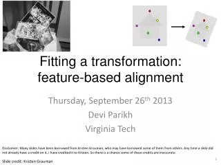
Alignment problem • We have previously considered how to fit a model to image evidence • e.g., a line to edge points, or a snake to a deforming contour • In alignment, we will fit the parameters of some transformation according to a set of matching feature pairs (“correspondences”). xi ' xi T Slide credit: Kristen Grauman
Parametric (global) warping • Examples of parametric warps: aspect rotation translation perspective affine Source: Alyosha Efros
T Parametric (global) warping • Transformation T is a coordinate-changing machine: • p’ = T(p) • What does it mean that T is global? • Is the same for any point p • can be described by just a few numbers (parameters) • Let’s represent T as a matrix: • p’ = Mp p = (x,y) p’ = (x’,y’) Source: Alyosha Efros
Scaling • Scaling a coordinate means multiplying each of its components by a scalar • Uniform scaling means this scalar is the same for all components: 2 Source: Alyosha Efros
X 2,Y 0.5 Scaling • Non-uniform scaling: different scalars per component: Source: Alyosha Efros
Scaling • Scaling operation: • Or, in matrix form: scaling matrix S Source: Alyosha Efros
What transformations can be represented with a 2x2 matrix? 2D Scaling? 2D Rotate around (0,0)? 2D Shear? Source: Alyosha Efros
What transformations can be represented with a 2x2 matrix? 2D Mirror about Y axis? 2D Mirror over (0,0)? 2D Translation? NO! Source: Alyosha Efros
2D Linear Transformations • Only linear 2D transformations can be represented with a 2x2 matrix. • Linear transformations are combinations of … • Scale, • Rotation, • Shear, and • Mirror Source: Alyosha Efros
Homogeneous coordinates To convert to homogeneous coordinates: homogeneous image coordinates Converting from homogeneous coordinates Slide credit: Kristen Grauman
Homogeneous Coordinates • Q: How can we represent 2d translation as a 3x3 matrix using homogeneous coordinates? • A: Using the rightmost column: Source: Alyosha Efros
Translation Homogeneous Coordinates tx = 2ty= 1 Source: Alyosha Efros
Basic 2D Transformations • Basic 2D transformations as 3x3 matrices Translate Scale Rotate Shear Source: Alyosha Efros
2D Affine Transformations • Affine transformations are combinations of … • Linear transformations, and • Translations • Parallel lines remain parallel Slide credit: Kristen Grauman
Today • Interactive segmentation • Feature-based alignment • 2D transformations • Affine fit • RANSAC Slide credit: Kristen Grauman
Alignment problem • We have previously considered how to fit a model to image evidence • e.g., a line to edge points, or a snake to a deforming contour • In alignment, we will fit the parameters of some transformation according to a set of matching feature pairs (“correspondences”). xi ' xi T Kristen Grauman
Image alignment • Two broad approaches: • Direct (pixel-based) alignment • Search for alignment where most pixels agree • Feature-based alignment • Search for alignment where extracted features agree • Can be verified using pixel-based alignment Slide credit: Kristen Grauman
Fitting an affine transformation • Assuming we know the correspondences, how do we get the transformation? Slide credit: Kristen Grauman
An aside: Least Squares Example • Say we have a set of data points (X1,X1’), (X2,X2’), (X3,X3’), etc. (e.g. person’s height vs. weight) • We want a nice compact formula (a line) to predict X’s from Xs: Xa + b = X’ • We want to find a and b • How many (X,X’) pairs do we need? • What if the data is noisy? Ax=B overconstrained Source: Alyosha Efros
Fitting an affine transformation • Assuming we know the correspondences, how do we get the transformation? Slide credit: Kristen Grauman
Fitting an affine transformation • How many matches (correspondence pairs) do we need to solve for the transformation parameters? • Once we have solved for the parameters, how do we compute the coordinates of the corresponding point for ? • Where do the matches come from? Kristen Grauman
What are the correspondences? ? • Compare content in local patches, find best matches. • e.g., simplest approach: scan with template, and compute SSD or correlation between list of pixel intensities in the patch • Later in the course: how to select regions according to the geometric changes, and more robust descriptors. Kristen Grauman
Fitting an affine transformation Affine model approximates perspective projection of planar objects. Figures from David Lowe, ICCV 1999 Slide credit: Kristen Grauman
Today • Interactive segmentation • Feature-based alignment • 2D transformations • Affine fit • RANSAC Slide credit: Kristen Grauman
Outliers • Outliers can hurt the quality of our parameter estimates, e.g., • an erroneous pair of matching points from two images • an edge point that is noise, or doesn’t belong to the line we are fitting. Kristen Grauman
Outliers affect least squares fit Slide credit: Kristen Grauman
