Feature Transformation and Normalization
Feature Transformation and Normalization. Reference : Springer Handbook of Speech Processing, 3.3 Environment Robustness (J. Droppo , A. Acero ). Present by Howard. Feature Moment Normalization.

Feature Transformation and Normalization
E N D
Presentation Transcript
Feature Transformation and Normalization Reference : Springer Handbook of Speech Processing, 3.3 Environment Robustness (J. Droppo, A. Acero) Present by Howard
Feature Moment Normalization The goal of feature normalization is to apply a transformation to the incoming observation features. This transformation should eliminate variabilities unrelated to the transcription. Even if you do not know how the ASR features have been corrupted, it is possible to normalize them to reduce the effects of the corruption. Techniques using this approach include cepstral mean normalization, cepstral mean and variance normalization, and cepstral histogram normalization.
Automatic Gain Normalization • Another type of normalization affects only the energy-like • features of each frame. • Automatic gain normalization (AGN) is used to ensure that the • speech occurs at the same absolute signal level, regardless of the • incoming level of background noise or SNR. • it is sometimes beneficial to use AGN on the energy-like features, • and the more-general moment normalization on the rest.
Cepstral Mean Normalization • Cepstralmean normalization consists of subtracting the mean • feature vector μ from each vector x to obtain the normalized • vector. • As a result, the long-term average of any observation sequence • (the first moment) is zero.
Cepstral Mean Normalization • As long as these convolutional distortions have a time constant • that is short with respect to the front end’s analysis window • length, and does not suppress large regions of the spectrum • below the noise floor (e.g., a severe low-pass filter), CMN can • virtually eliminate their effects. • As the filter length h[m] grows, becomes less accurate and CMN • is less effective in removing the convolutional distortion.
CMN VS. AGN • Inmost cases, using AGNis better than applying CMN on the • energy term. • The failure of CMN on the energy feature is most likely due to • the randomness it induces on the energy of noisy speech frames. • AGN tends to put noisy speech at the same level regardless of • SNR, which helps the recognizer make sharp models. • On the other hand, CMN will make the energy term smaller in • low-SNR utterances and larger in high-SNR utterances, leading • to less-effective speech models.
CMN VS. AGN in different stages • One option is to use CMN on the static cepstra, before • computing the dynamic cepstra. Because of the nature of CMN, • this is equivalent to leaving the dynamic cepstra untouched. • The other option is to use CMN on the full feature vector, after • dynamic cepstra have been computed from the unnormalized • static cepstra. • The following table shows that it is slightly better to apply • the normalization to the full feature vectors.
Cepstral Variance Normalization • Cepstral variance normalization (CVN) is similar to CMN, and • the two are often paired as cepstral mean and variance • normalization (CMVN). • CMVN uses both the sample mean and standard deviation to • normalize the cepstral sequence: • After normalization, the mean of the cepstral sequence is zero, • and it has a variance of one.
Cepstral Variance Normalization • UnlikeCMN, CVNis not associated with addressing a particular • type of distortion. It can, however, be shown empirically that it • provides robustness against acoustic channels, speaker • variability, and additive noise. • As with CMN, CMVN is best applied to the full feature vector, • after the dynamic cepstra have been computed. Unlike CMN, the • tables show that applying CMVN to the energy term is often • better than using whole-utterance AGN.
Cepstral Variance Normalization • Unlike CMN, the tables show that applying CMVN to the energy • term is often better than using whole-utterance AGN. Because • CMVN is both shifting and scaling the energy term, both the • noisy speech and the noise are placed at a consistent absolute • levels.
Cepstral Histogram Normalization • Cepstral histogram normalization (CHN) takes the core ideas • behind CMN and CVN, and extends them to their logical • conclusion. • Instead of only normalizing the first or second central moments, • CHN modifies the signal such that all of its moments are • normalized. • As with CMN and CHN, a one-to-one transformation is • independently applied to each dimension of the feature vector.
Cepstral Histogram Normalization • The first step in CHN is choosing a desired distribution for the • data, . It is common to choose a Gaussian distribution with • zero mean and unit covariance. • Let represent the actual distribution of the data to be • transformed. • It can be shown that the following function f (·) applied to y • produces features with the probability distribution function • (PDF) px (x): • Here, Fy(y) is the cumulative distribution function (CDF) of the • test data.
Cepstral Histogram Normalization • Applying Fy(·) to y transforms the data distribution from py(y) to • a uniform distribution. • Subsequent application of (·) imposes a final distribution • of px (x). • When the target distribution is chosen to be Gaussian as • described above, the final sequence has zero mean and unit • covariance, just as if CMVN were used. • First, the data is transformed so it has a uniform distribution.
Cepstral Histogram Normalization • The second and final step consists of transforming so that • it has a Gaussian distribution. This can be accomplished, as in • (33.11), using an inverse Gaussian CDF :
Analysis of Feature Normalization • When implementing feature normalization, it is very important to • use enough data to support the chosen technique. • If test utterances are too short to support the chosen • normalization technique, degradation will be most apparent in • the clean-speech recognition results. • In cases where there is not enough data to support CMN, Rahim • has shown that using the recognizer’s acoustic model to estimate • a maximum-likelihood mean normalization is superior to • conventional CMN.
Analysis of Feature Normalization • It has been found that CMN does not degrade the recognition • rate on utterances from the same acoustical environment, as long • as there are at least four seconds of speech frames available. • CMVN and CHN require even longer segments of speech. • When a system is trained on one microphone and tested on • another, CMN can provide significant robustness. • Interestingly, it has been found in practice that the error rate for • utterances within the same environment can actually be • somewhat lower. This is surprising, given that there is no • mismatch in channel conditions.
Analysis of Feature Normalization • One explanation is that, even for the same microphone and room • acoustics, the distance between the mouth and the microphone • varies for different speakers, which causes slightly different • transfer functions. • The cepstral mean characterizes not only the channel transfer • function, but also the average frequency response of different • speakers. By removing the long-term speaker average, CMN can • act as sort of speaker normalization. • One drawback of CMN, CMVN, and CHN is that they do not • discriminate between nonspeech and speech frames in • computing the utterance mean.
Analysis of Feature Normalization • For instance, the mean cepstrum of an utterance that has 90% • nonspeech frames will be significantly different from one that • contains only 10% nonspeech frames. • An extension to CMN that addresses this problem consists in • computing different means for noise and speech. • Speech/noise discrimination could be done by classifying frames • into speech frames and noise frames, computing the average • cepstra for each, and subtracting them from the average in the • training data.
My Experiment and observation • They are both mean normalization wethods, why is AGN better than CMN ? • Because the maximum c0 must contain noise? It not only • remove convolution but also the most noise, and that’s why • is can just used on the log energy term. • Why CMVN is better than both of CMN and AGN, even if we • just use CMVN on energy term while use AGN and CMN to full • MFCC ? • Because variance normalization on energy term has the • most contribution. The energy term reacts the whole • energy and contains the maximum vanriance.
My Experiment and observation • Both of CMVN and CHN have assumption of following • Gaussian distribution with . • They are the same in term of distribution. • What’s different ? • CMVN uses linear transformation to complete Gaussian • distribution, but CHN gets it through nonlinear • transformation of Gaussian distribution. • Is there no miss information in CMVN? • The data sparseness is more sever in CMVN.
My Experiment and observation • CMVN • Std dev >1 • The more near to mean, the more is left. • The more far from mean, the more is subtracted. • The distribution changes form fat and short to tall • and thin. • Std dev <1 • The more near to mean, the less is enlarged. • The more far from mean, the more is enlarged. • The distribution changes form tall and thin to short • and fat.
Question • Is it good for contain smaller variance? • The range of value to PCA should be smaller? • The sharp acoustic model is good?
Idea • Use multi data to train a good variance. • Map multi cdf to clean MFCC • Shift mean of test data to recognize.