SURVIVAL ANALYSIS
SURVIVAL ANALYSIS. Development Workshop. What is endogeneity and why we do not like it? [REPETITION]. Three causes: X influences Y, but Y reinforces X too Z causes both X and Y fairly contemporaneusly

SURVIVAL ANALYSIS
E N D
Presentation Transcript
SURVIVAL ANALYSIS Development Workshop
What is endogeneity and why we do not like it? [REPETITION] • Three causes: • X influences Y, but Y reinforces X too • Z causes both X and Y fairly contemporaneusly • X causes Y, but we cannot observe X and Z (which we observe) is influenced by X but also by Y • Consequences: • No matter how many observations – estimators biased (this is called: inconsistent) • Ergo: whatever point estimates we find, we can’t even tell if they are positive/negative/significant, because we do not know the size of bias + no way to estimate the size of bias
The mystery of staying alive T t0 t1 t2 t3 ...... tN • Everything started in medicine and biology • Key question: can we talk about determinants of survival from t1 to t2, knowing at least that part of people survived from t0 to t1? • No magic sticks, cannot „guess” future, but • Surviving till time T, means S(T) = P(Y>T) • We can estimate P(Y>T) on our sample (what is random here?) • Time is discrete (eventually there is nobody left to die…) • P(surviving till T) = S(T) = P(Y>T)= p(t1) ·p(t2) ·... ·p(tN)
Technically speaking • Each period we may estimate a probit of surviving till t if I am still alive in t-1 P(live in t | survived till t-1) • De facto, this is a sequence of estimation p(live_t|live_t-1), p(live_t+1|live_t), p(live_t+2|live_t+1), etc. • For each ti we may specify: • ni-1– no of people at risk in ti-1, i.e. „momentarily earlier” • di – no of people who disappeared from the sample between ti-1 and ti ni = ni-1 – di, n0=N • Probability of staying alove between ti-1 and ti: p(ti) = P(ti|Y>ti-1) = (ni-1 – di)/ni-1 = 1 – di/ni-1
Clinical data 20 observations, 10 deaths, 10 censored observations (people still alive when observation window has ended) Observation period (FU) counted in months since treatment ended Example
Kaplan-Meier estimator t0=0 t1=2.3655 n0=20 d1=1, c1=0 n1 = 20 – 1 =19 S(t1) = P(Y>t1) = P(t1|Y>t0)*P(Y>t0) = (1- 1/20)*1=0.95
Kaplan-Meier estimator t18=19.7043 t19=21.9425 n18=2 d19=1, c19=0 n19 = 2 – 1 =1 S(t19)=P(Y>t19) = P(t19|Y>t18)*P(Y>t18) = (1- 1/2)*0.3863 = 0.5*0.39=0.19
Additional pitfalls • Assume that survival is conditional on something (not just numbers thrown now and then) • Crucial assumption: distribution of survival • Exponential: λ(t)= λ /constant with the sample?/ • Weibull: λ(t) = λpptp-1 /variable, but how?/ • Gompertz-Makeham: λ(t) = e{α+βt} /also variable…? / • Gamma: S(t) = 1 - Ik(λ t) /also variable…? / • A whole variety…
Pros and cons of KM estimator • Advantages: • Intuitive • Little data needs • Computed on data (always can get it) • Disadvantages: • Cannot know if some characteristics help/inhibit survival • No tests, statistical hypotheses, etc. • Overall: nice drawing tool, poor analytical tool => need an analytical tool
Other similar estimators • Nelson-Aalena • Similar to KM – starts from hazard functions and not survival function • Computed on data – nothing more than visualisation • You could test for two (or more) groups as well • Mantel-Haenszel • If probability of death was similar across two groups, no of observations still alive at each point in time should keep the same proportion => testable • Cox • Combinations of different tests
Cox model Define h(t) – hazard function probability of dying at t if you survived untill t x1, x2, ..., xk – set of hazard factors h0(t) – base hazard function in base group, t – observation time β1, β 2, ..., β k – coefficients of model b × = 1 h ( t ) e h ( t , x 1 ) b = = 0 e b × = 0 h ( t , x 0 ) h ( t ) e 0 comparedgroups
Pros and cons for Cox model Disadvantages: the quotient for the hazard funcitons CONSTANT OVER TIME ! no (direct) information on h0(t) simple hypotheses only (are two groups different) Advantages graphical test: curves of ln(-ln(S(t)) for groups compared can condition some characteristics Frailty – a big issue
How do we do this in STATA? 14 • Survival functions twoway line S age • Hazard functions gen H = - log(S) gen h = H[_n] - H[_n-1] gen logh = log(h) gen agem = age - 0.5 if h <. twoway line logh agem, xtitle("age")
How do we do this in STATA? 2011-05-12 Seminarium magisterskie - zajęcia 7 15 • Generally, two approaches: • From data (nonparametric) stscox, stsgraph • Assuming something about hazard distribution (parametric) stsreg, stscurve • First have to declare data to have survival form: • Variable declaring „death” + variable declaring „time” stset time, failure(death)
How do we do this in STATA? • Parametrically stset time, fail(death) streg all_conditioning_variables, distribution(your_selected_distribution) • Nonparametrically sts graph /Kaplan Meier/ sts graph, by(group) /Kaplan Meier/ sts test group /Mantel-Haenszel/ stcox group /Cox/ stphtest, plot(group) /testing whether we can use Cox model/ stphplot, by(treated) /graphical confirmation for the PH test/ • And that’s all, folks
Summary Not a very sophisticated tool How sophisticated question – depends on us With large samples – nonparametric methods have some serious edge to rely on If samples small – parametric methods may be less reliable How about „direction of causality” here? Do we run the risk of endogeneity bias?

