Survival Analysis

1. Survival Analysis A Brief Introduction

3. 1. SurvivalFunction, Hazard Function • In many medical studies, the primary endpoint is time until an event occurs (e.g. death, remission) • Data are typically subject to censoring (e.g. when a study ends before the event occurs) • Survival Function - A function describing the proportion of individuals surviving to or beyond a given time. Notation: • T: survival time of a randomly selected individual • t: a specific point in time. • Survival Function:

4. Hazard Function/Rate • Hazard Function l(t): instantaneous failure rate at time t given that the subject has survived upto time t. That is • Here f(t) is the probability density function of the survival time T. That is, • where F(t) is the cumulative distribution function of T: 4

5. 2. The Key Word is ‘Censoring’ • Because of censoring, many common data analysis procedures can not be adopted directly. • For example, one could use the logistic regression model to model the relationship between survival probability and some relevant covariates • However one should use the customized logistic regression procedures designed to account for censoring 5

6. Key Assumption: Independent Censoring • Those still at risk at time t in the study are a random sample of the population at risk at time t, for all t • This assumption means that the hazard function, λ(t), can be estimated in a fair/unbiased/valid way

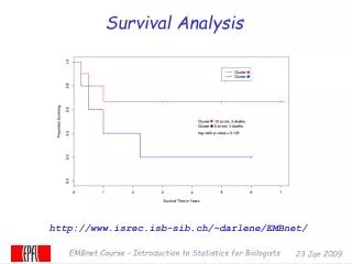
7. 3A. Kaplan-Meier (Product-Limit) Estimator of the Survival Curve • The Kaplan–Meier estimator is the nonparametric maximum likelihood estimate of S(t). It is a product of the form • is the number of subjects alive just before time • denotes the number who died at time

8. Kaplan-Meier Curve, Example

9. Kaplan Meier Curve 9

10. Figure 1. Plot of survival distribution functions for the NCI and the SCI Groups. The Y-axis is the probability of not declining to GDS 3 or above. The X-axis is the time (in years) to decline. (Barry Reisberg et al., 2010; Alzheimer & Dementia; in press.)

11. 3B. Comparing Survival Functions 1.00 0.75 High Survival Distribution Function 0.50 Low 0.25 Medium 0.00 0 10 20 30 40 50 60 Time

12. Log-Rank Test • The log-rank test • tests whether the survival functions are statistically equivalent • is a large-sample chi-square test that uses the observed and expected cell counts across the event times • has maximum power when the ratio of hazards is constant over time.

13. Wilcoxon Test • The Wilcoxon test • weights the observed number of events minus the expected number of events by the number at risk across the event times • can be biased if the pattern of censoring is different between the groups.

14. Log-rank versus Wilcoxon Test • Log-rank test • is more sensitive than the Wilcoxon test to differences between groups in later points in time. • Wilcoxon test • is more sensitive than the log-rank test to differences between groups that occur in early points in time.

15. 4. Two Parametric Distributions • Here we present two most notable models for the distribution of T. • Exponential distribution: • Weibull distribution: • Its survival function: • Thus:

16. Weibull Hazard Function, Plot

17. 5. Regression Models • The Exponential and the Weibull distribution inspired two parametric regression approaches: • Parametric proportional hazard model – this model can be generalized to a semi-parametric model: the Cox proportional hazard model • Accelerated failure time model

18. Proportional Hazard Model • In a regression model for survival analysis one can try to model the dependence on the explanatory variables by taking the (new) hazard rate to be: • Hazard rates being positive it is natural to choose the function c such that c(β,x) is positive irrespective the values of x.

19. Proportional Hazard Model • Thus a good choice is: • The resulting proportional hazard model is: • For the Weibull distribution we have: • For the Exponential distribution we have:

20. Accelerated Failure Time Model • For the Weibull distribution (including the Exponential distribution), the proportional hazard model is equivalent to a log linear model in survival time T: • Here the error term can be shown to follow the 2-parameter Extreme Vvalue distribution

21. Apply Both Models Simultaneously • If the underlying distribution for T is Weibull or Exponential, one can apply both regression models simultaneously to reflect different aspects of the survival process. That is • Prediction of degree of decline using the Weibull proportional hazard model • Prediction of time of decline using the accelerated failure time model

22. An Example • In a recent paper (Reisberg et al., 2010), we applied both regression models to a dementia study conducted at NYU: • The results are shown next

24. 6. Cox Proportional Hazards Model

25. Parametric versus Nonparametric Models • Parametric models require that • the distribution of survival time is known • the hazard function is completely specified except for the values of the unknown parameters. • Examples include the Weibull model, the exponential model, and the log-normal model.

26. Parametric versus Nonparametric Models • Properties of nonparametric models are • the distribution of survival time is unknown • the hazard function is unspecified. • An example is the Cox proportional hazards model.

27. ... Linear function of a set of predictor variables - does not involve time Baseline Hazard function - involves time but not predictor variables Cox Proportional Hazards Model • β = 0 → hazard ratio = 1 • Two groups have the same survival experience

28. Popularity of the Cox Model • The Cox proportional hazards model • provides the primary information desired from a survival analysis, hazard ratios and adjusted survival curves, with a minimum number of assumptions • is a robust model where the regression coefficients closely approximate the results from the correct parametric model.

29. Partial Likelihood • Partial likelihood differs from maximum likelihood because • it does not use the likelihoods for all subjects • it only considers likelihoods for subjects that experience the event • it considers subjects as part of the risk set until they are censored.

30. Partial Likelihood Subject Survival Time Status C 2.0 1 B 3.0 1 A 4.0 0 D 5.0 1 E 6.0 0

31. Partial Likelihood

32. Partial Likelihood

33. Partial Likelihood • The overall likelihood is the product of the individual likelihood. That is:

34. 7. SAS Programs for Survival Analysis • There are three SAS procedures for analyzing survival data: LIFETEST, PHREG, and LIFEREG. • PROC LIFETEST is a nonparametric procedure for estimating the survivor function, comparing the underlying survival curves of two or more samples, and testing the association of survival time with other variables. • PROC PHREG is a semiparametric procedure that fits the Cox proportional hazards model and its extensions. • PROC LIFEREG is a parametric regression procedure for modeling the distribution of survival time with a set of concomitant variables.

35. Proc LIFETEST • The Kaplan-Meier(K-M) survival curves and related tests (Log-Rank, Wilcoxon) can be generated using SAS PROC LIFETEST PROC LIFETEST DATA=SAS-data-set <options>; TIME variable <*censor(list)>; STRATA variable<(list)> <...variable <(list)>>; TEST variables; RUN;

36. Proc PHREG The Cox (proportional hazards) regression is performed using SAS PROC PHREG proc phreg data=rsmodel.colon; model surv_mm*status(0,2,4) = sex yydx / risklimits; run;

37. Proc LIFEREG • The accelerated failure time regression is performed using SAS PROC LIFEREG proc lifereg data=subset outest=OUTEST(keep=_scale_); model (lower, hours) = yrs_ed yrs_exp / d=normal; output out=OUT xbeta=Xbeta; run;

38. Selected References • PD Allison (1995). Survival Analysis Using SAS: A Practical Guide. SAS Publishing. • JD Kalbfleisch and RL Prentice (2002).The Statistical Analysis of Failure Time Data. Wiley-Interscience.

39. Questions?