Download
1 / 23
230 likes | 373 Vues
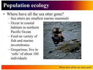
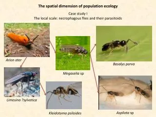
The spatial dimension of population ecology. Case study I The local scale: necrophagous flies and their parasitoids. Arion ater. Basalys parva. Megaselia sp. Limosina ?sylvatica. Aspilota sp. Kleidotoma psiloides. The spatial distribution of individuals. Photo Polystyrol.

E N D
The spatial dimension of population ecology Case study I The local scale: necrophagous flies and their parasitoids Arion ater Basalys parva Megaseliasp Limosina ?sylvatica Aspilota sp Kleidotoma psiloides
The spatial distribution of individuals Photo Polystyrol Each slug was covered by a beech leaf Does spatial distribution change with abundance? Do parasitoids and hosts differ in spatial distribution? Is spatial distribution linked to resource availability? Does spatial distribution contributes to population stability? 100 boxes arranged in a regular 10x10 m grid each with a dead slug What is the spatial distribution of flies, parasitoids, and hyperparasitoids
The sequence of colonisation The limiting factor of colonisation was carcass desiccation Desiccation is dependent on plant cover
Coniceraschnittmanni Megaselia sp1 Aspilota sp1 Orthostigma sp1
Aspilotasp1 Orthostigmasp1 Kleidotomapsiloides Aspilotasp1
Spatial aggregation Coefficient of variation Morisita index Mean crowding (Lloyd index) N denote the occasions in each of the N sites. Poisson random distribution Poisson random: J = 1 Regular (segregated, overdispersed): J << 1 Clumped (aggregated, underdispersed): J >> 1 Statistical inference has to come from a Monte Carlo ranodmisation.
Lloyd index and species abundances Parasitoids Diptera • Necrophagous flies and their parasitoids : • Highly aggregated • Aggregation decreases with average abundance • Both guilds have the same degree of aggregation
Spatialsegregation of species? Table of Pearson correlations (lower triangle) and the respectivesignificancelevels (upper triangle)
Biplots of principal component analyses Limosina sp PCA separates sphaerocerid species from C. schnittmanni and the other phorid species C. schnittmanni Aspilota sp1 PCA separates the abundant Aspilota sp1 and sp2 K. psiloides Aspilota sp2
Differences in the populations of necrophages and theirparasitoids
Case study II The regional scale: fragmented landscapes and meta-populations Meta-populations refer to the spread of local populations of a single species within a fragmented landscape. Local populations are connected by dispersal Questions: Minimum fragment size Minimum dispersal rate for survival Percentage of fragments colonised Speed of genetic divergence within fragments What is the influence of fragment edges? How do corridors influence dispersal rates?
Case study II The regional scale: fragmented landscapes and meta-populations The Lotka – Volterra model of population growth The spatial distribution of species is scattered among isolated fragments. Fragments differ in population size Levins (1969) assumed that the change in the occupancy of single spatially separated habitats (islands) follows the same model. Assume P being the number of islands (total K) occupied. Q= K-P is then the proportion of not occupied islands. m is the immigration and e the local extinction probability. Distance Emigration/Extinction Colonisations The Levins model of meta-populations The higher the population size is, the lower is the local extinction probability and the higher is the emigration rate
If we deal with the fraction p of fragments colonized The canonical model of metapopulation ecology Metapopulation modelling allows for an estimation of species survival in fragmented landscapes and provides estimates on species occurrences. Colonisation probability is exponentially dependent on the average distance I of the islands and extinction probability scales proportionally to island size. The standard equation of metapopulationmodeling
Extinction times If we know local extinction times TL we can estimate the regional time TR to extinction When is a metapopulation stable? 1200 1000 800 Median time to extinction 600 400 The meta-population is only stable if m > e. 200 0 0 1 2 3 4 5 6 7 0.5 If m and e are known p denotes the proportion of fragments colonised p K The condition for long-term survival
Bird metapopulations Zosteropspoliogaster Zosteropsabyssinicus The lowland Z. abyssinicushas a continuous distribution. The highland Z. poliogaster has a scattered mountain distribution. It has a meta-population structure. The highland species occurs in forest fragments
Morphological raw data Bird call raw data Allele frequency raw data Data collected by J. C. Habel, TH Munich
ANOVA probabilities for no difference Bird call patterns Local birdcalls within Z. poliogaster are more different than between Z. poliogaster and Z. abyssinicus Birdcall within the lowland Z. poliogasterdo not significantly differ
: Bird calls: Allele frequencies : Morphology Bird call patterns within Z. poliogaster differ more between local populations than do genetic and morphological charcters. Northern and southern populations of Z. poliogaster differ considerable in bird dialect. Soon gen flow will cease despite of occasional migration.
Geographic distances in m The average relative distance of a site to all other sites. Species population occupancy modelling SPOM a = 0.5b = 0.5c = 1
Species population occupancy modelling SPOM High dispersal increases theprobability of occupancy. High local mortality decreases local colonisation. Distance between fragments has a high impact on colonisation probability. The highly isolated Mt. Kulal has low occupancy probabilities. For long-term stability of the meta-population at least 77% = 12 sites have to be occupied 3/√15 = 0.77
Is the species endangered? The loss of habitats might provide to fast extinction Zosteropspoliogaster is regionally not endangered despite of the higher local extinction probabilities