Download
1 / 55
550 likes | 712 Vues
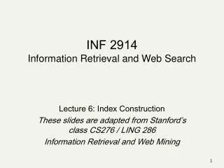
INF 2914 Information Retrieval and Web Search. Lecture 6: Index Construction These slides are adapted from Stanford’s class CS276 / LING 286 Information Retrieval and Web Mining. (Offline) Search Engine Data Flow. Parse & Tokenize. Global Analysis. Index Build. Crawler. Dup detection

E N D
INF 2914Information Retrieval and Web Search Lecture 6: Index Construction These slides are adapted from Stanford’s class CS276 / LING 286 Information Retrieval and Web Mining
(Offline) Search Engine Data Flow Parse & Tokenize Global Analysis Index Build Crawler • Dup detection • Static rank • Anchor text • Spam analysis • - … - Scan tokenized web pages, anchor text, etc- Generate text index web page - Parse- Tokenize- Per page analysis 1 2 3 4 in background duptable tokenizedweb pages anchortext ranktable spam table invertedtext index
Brutus Calpurnia Caesar Dictionary Postings lists Inverted index • For each term T, we must store a list of all documents that contain T. Posting 2 4 8 16 32 64 128 1 2 3 5 8 13 21 34 13 16 Sorted by docID (more later on why).
Tokenizer Friends Romans Countrymen Token stream. Linguistic modules friend friend roman countryman Modified tokens. roman Indexer 2 4 countryman 1 2 Inverted index. 16 13 Inverted index construction Documents to be indexed. Friends, Romans, countrymen.
Indexer steps • Sequence of (Modified token, Document ID) pairs. Doc 1 Doc 2 I did enact Julius Caesar I was killed i' the Capitol; Brutus killed me. So let it be with Caesar. The noble Brutus hath told you Caesar was ambitious
Sort by terms. Core indexing step.
Multiple term entries in a single document are merged. • Frequency information is added. Why frequency? Will discuss later.
The result is split into a Dictionary file and a Postings file.
The index we just built • How do we process a query?
2 4 8 16 32 64 1 2 3 5 8 13 21 Query processing: AND • Consider processing the query: BrutusANDCaesar • Locate Brutus in the Dictionary; • Retrieve its postings. • Locate Caesar in the Dictionary; • Retrieve its postings. • “Merge” the two postings: 128 Brutus Caesar 34
Brutus Caesar 13 128 2 2 4 4 8 8 16 16 32 32 64 64 8 1 1 2 2 3 3 5 5 8 8 21 21 13 34 The merge • Walk through the two postings simultaneously, in time linear in the total number of postings entries 128 2 34 If the list lengths are x and y, the merge takes O(x+y) operations. Crucial: postings sorted by docID.
Index construction • How do we construct an index? • What strategies can we use with limited main memory?
Our corpus for this lecture • Number of docs = n = 1M • Each doc has 1K terms • Number of distinct terms = m = 500K • 667 million postings entries
How many postings? • Number of 1’s in the i th block = nJ/i • Summing this over m/J blocks, we have • For our numbers, this should be about 667 million postings.
Recall index construction • Documents are processed to extract words and these are saved with the Document ID. Doc 1 Doc 2 I did enact Julius Caesar I was killed i' the Capitol; Brutus killed me. So let it be with Caesar. The noble Brutus hath told you Caesar was ambitious
Key step • After all documents have been processed the inverted file is sorted by terms. We focus on this sort step. We have 667M items to sort.
Index construction • At 10-12 bytes per postings entry, demands several temporary gigabytes
System parameters for design • Disk seek ~ 10 milliseconds • Block transfer from disk ~ 1 microsecond per byte (following a seek) • All other ops ~ 1 microsecond • E.g., compare two postings entries and decide their merge order
Bottleneck • Build postings entries one doc at a time • Now sort postings entries by term (then by doc within each term) • Doing this with random disk seeks would be too slow – must sort N=667M records If every comparison took 2 disk seeks, and N items could be sorted with N log2N comparisons, how long would this take?
Disk-based sorting Build postings entries one doc at a time Now sort postings entries by term Doing this with random disk seeks would be too slow – must sort N=667M records If every comparison took 2 disk seeks, and N items could be sorted with N log2N comparisons, how long would this take? 12.4 years!!! 20
Sorting with fewer disk seeks 12-byte (4+4+4) records (term, doc, freq). These are generated as we process docs. Must now sort 667M such 12-byte records by term. Define a Block ~ 10M such records can “easily” fit a couple into memory. Will have 64 such blocks to start with. Will sort within blocks first, then merge the blocks into one long sorted order. 21
Sorting 64 blocks of 10M records First, read each block and sort within: Quicksort takes 2N ln N expected steps In our case 2 x (10M ln 10M) steps Time to Quicksort each block = 320 seconds Total time to read each block from disk and write it back 120M x 2 x 10-6 = 240 seconds 64 times this estimate - gives us 64 sorted runs of 10M records each Total Quicksort time = 5.6 hours Total read+write time = 4.2 hours Total for this phase ~ 10 hours Need 2 copies of data on disk, throughout 22
Merging 64 sorted runs Merge tree of log264= 6 layers. During each layer, read into memory runs in blocks of 10M, merge, write back. 1 3 2 4 2 1 Merged run. 3 4 Runs being merged. Disk 23
Merge tree 1 run … ? 2 runs … ? 4 runs … ? 8 runs, 80M/run 16 runs, 40M/run … 32 runs, 20M/run Bottom level of tree. Sorted runs. … 1 2 63 64 24
Merging 64 runs Time estimate for disk transfer: 6 x Time to read+write 64 blocks = 6 x 4.2 hours ~ 25 hours Time estimate for the merge operation: 6 x 640M x 10-6 = 1 hour Time estimate for the overall algorithm: Sort time + Merge time ~ 10 + 26 ~ 36 hours Lower bound (main memory sort): Time to read+write = 4.2 hours Time to sort in memory = 10.7 hours Total time ~ 15 hours 25
How to improve indexing time? Compression of the sorted runs Multi-way merge Heap merge all runs Radix sort (linear time sorting) Pipelining reading, sorting, and writing phases 27
Multi-way merge Heap Sorted runs … 1 2 63 64 28
Indexing improvements Radix sort Linear time sorting Flexibility in defining the sort criteria Bigger sort buffers increase performance (contradicting previous literature) (see VLDB paper on the references) Pipelining read and sort + write phases B1 B1 B1 B1 Read B2 B2 B2 B2 Sort + Write time 29
Positional indexing Given documents:D1: This is a testD2: Is this a testD3: This is not a test Reorganize by term: TERM DOC LOC DATA(caps)this 1 0 1is 1 1 0a 1 2 0test 1 3 0is 2 0 1this 2 1 0a 2 2 0test 2 3 0this 3 0 1is 3 1 0not 3 2 0a 3 3 0test 3 4 0 30
Positional indexing In “postings list” format: a (1,2,0),(2,2,0),(3,3,0) is (1,1,0),(2,0,1),(3,1,0) not (3,2,0) test (1,3,0),(2,3,0),(3,4,0) this (1,0,1),(2,1,0),(3,0,1) Sort by <term, doc, loc>: TERM DOC LOC DATA(caps)a 1 2 0a 2 2 0a 3 3 0is 1 1 0is 2 0 1is 3 1 0not 3 2 0 test 1 3 0test 2 3 0test 3 4 0 this 1 0 1 this 2 1 0 this 3 0 1 31
Positional indexing with radix sort Radix key = Token hash = 8 bytes Document ID = 8 bytes Location = 4 bytes, but no need to sort by location since Radix sort is stable! 32
Distributed indexing Maintain a master machine directing the indexing job – considered “safe” Break up indexing into sets of (parallel) tasks Master machine assigns each task to an idle machine from a pool 33
Parallel tasks We will use two sets of parallel tasks Parsers Inverters Break the input document corpus into splits Each split is a subset of documents Master assigns a split to an idle parser machine Parser reads a document at a time and emits (term, doc) pairs 34
Parallel tasks Parser writes pairs into j partitions Each for a range of terms’ first letters (e.g., a-f, g-p, q-z) – here j=3. Now to complete the index inversion 35
Data flow Master assign assign Postings Parser Inverter a-f g-p q-z a-f Parser a-f g-p q-z Inverter g-p Inverter splits q-z Parser a-f g-p q-z 36
Inverters Collect all (term, doc) pairs for a partition Sorts and writes to postings list Each partition contains a set of postings Above process flow a special case of MapReduce. 37
MapReduce Model for processing large data sets. Contains Map and Reduce functions. Runs on a large cluster of machines. A lot of MapReduce programs are executed on Google’s cluster everyday. 38
Motivation Input data is large The whole Web, billions of Pages Lots of machines Use them efficiently 39
A real example Term frequencies through the whole Web repository. Count of URL access frequency. Reverse web-link graph …. 40
Programming model Input & Output: each a set of key/value pairs Programmer specifies two functions: map (in_key, in_value) -> list(out_key, intermediate_value) Processes input key/value pair Produces set of intermediate pairs reduce (out_key, list(intermediate_value)) -> list(out_value) Combines all intermediate values for a particular key Produces a set of merged output values (usually just one) 41
Example Page 1: the weather is good Page 2: today is good Page 3: good weather is good. 42
Example: Count word occurrences map(String input_key, String input_value): // input_key: document name // input_value: document contents for each word w in input_value: EmitIntermediate(w, "1"); reduce(String output_key, Iterator intermediate_values): // output_key: a word // output_values: a list of counts int result = 0; for each v in intermediate_values: result += ParseInt(v); Emit(AsString(result)); 43
Map output Worker 1: (the 1), (weather 1), (is 1), (good 1). Worker 2: (today 1), (is 1), (good 1). Worker 3: (good 1), (weather 1), (is 1), (good 1). 44
Reduce Input Worker 1: (the 1) Worker 2: (is 1), (is 1), (is 1) Worker 3: (weather 1), (weather 1) Worker 4: (today 1) Worker 5: (good 1), (good 1), (good 1), (good 1) 45
Reduce Output Worker 1: (the 1) Worker 2: (is 3) Worker 3: (weather 2) Worker 4: (today 1) Worker 5: (good 4) 46
Fault tolerance Typical cluster: 100s/1000s of 2-CPU x86 machines, 2-4 GB of memory Storage is on local IDE disks GFS: distributed file system manages data (SOSP'03) Job scheduling system: jobs made up of tasks, scheduler assigns tasks to machines Implementation is a C++ library linked into user programs) 49
Fault tolerance On worker failure: Detect failure via periodic heartbeats Re-execute completed and in-progress map tasks Re-execute in progress reduce tasks Task completion committed through master Master failure: Could handle, but don't yet (master failure unlikely) 50