STIFF: A Forecasting Framework for Spatio-Temporal Data

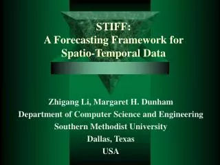
STIFF: A Forecasting Framework for Spatio-Temporal Data Zhigang Li, Margaret H. Dunham Department of Computer Science and Engineering Southern Methodist University Dallas, Texas USA

Our goal • In this paper, we present a novel forecasting framework for spatio-temporal data, in which not only spatial but also temporal characteristics of the data are considered to obtain a more appropriate result. Li & Dunham, PAKDD

Presentation Outline • Motivation • Prior Research • Our Approach: STIFF Combining two approaches to achieve better results: Time Series Analysis and ANNs • Performance • Future Work Li & Dunham, PAKDD

Why • There are many application fields which require spatio-temporal forecasting: • river hydrology, biological patterns, housing price research, rainfall distribution, waste monitoring, fishery, hotel pickup rate, etc. • In spatio-temporal forecasting, both spatial and temporal properties, as well as their mutual correlation, are taken into account. Li & Dunham, PAKDD

What work has been done • [Jothityangkoon, Sivapalan, and Viney, 2000] • Rainfall forecasting • Hidden Markov Model • De-aggregate high level to lower level • Large error • [Pokrajac and Obradovic,2001] • Current event assumed to be impacted only by immediate temporal ancestors. Li & Dunham, PAKDD

More related research • [Cressie and Majure,1997] • Model livestock waste in a river basin • Condensed time into a “three day area of influence” • “large variation of the predicted values”. • [Deutsch etal,1986]; [Kelly etal,1998]; [Pfeifer etal,1990] • Extended time series analysis with a spatial correlation from a simple distance matrix. • It is too arbitrary to just rely upon the pure distance measurement. Li & Dunham, PAKDD

Flood Forecasting (Our Motivating Application) • Catchment • Many different types of sensors • Predict at one sensor location • Water level or Flow rate • May not be interested in actual prediction of value Li & Dunham, PAKDD

Our approach : Problem definition • Δ={α0, α1, α2, … αn} is the research field, composed of n + 1 spatially separated subcomponents, named by αi accordingly. • WLOG, α0 is assumed the target place where forecasting is about to be carried out. • For each αi in Δ, there are j observations with equal time intervals between consecutive ones, denoted by Лi={αi1, αi2, αi3, … αij}. Li & Dunham, PAKDD

Problem definition (Cont.) • Given Δ={α0, α1, α2, … αn}, Л={Л1, Л2, …Лn}, the length of observations j and the look-ahead steps of ι, we are expected to find an as good as possible forecasting relationship ƒ that is defined as follows. Li & Dunham, PAKDD

Our approach : Algorithm sketch • Describe the forecasting problem according the problem definition. • Build a time series (ARIMA) model for each αi. Name the forecasting from α0 time series model as ƒT. • Construct and train an ANN to capture the spatial correlation and influence over the target subcomponent α0. Name the forecasting from the neural network as ƒS. • Combine ƒT and ƒS via a statistical regression mechanism. Li & Dunham, PAKDD

Time Series Data Transformation • Convert non-stationary to stationary to prevent skewness as much as possible. • Box and Cox proposed a transformation family, namely, Box-Cox transformation: • The key is to determine the right value for λ so as to find the appropriate transformation. For example, when λ = 0 or .5 the transformation is in fact log or square root accordingly. But how? Li & Dunham, PAKDD

Data transformation (cont’d) • Box and Cox proposed a large-sample maximum-likelihood approach. • Wei proposed to use the λ that minimizes • The former requires much computation while the latter one may incur some problems for it does not consider the difference compared to the real observation. • We therefore propose the following way to determine λ. Li & Dunham, PAKDD

Time series Model • A time series model is chosen as it has the proven capability of describing and capturing the temporal dependency and relationship. • Our work focused on the ARIMA technique which can be embodied in the following formula. • And roughly speaking, the building process can be divided into three main steps. They are • Model identification • Parameter estimation • Diagnostic checking Li & Dunham, PAKDD

Find the spatial influence • Normally it is much harder to find than its temporal counterpart in the problem. • No precise way to convert from the spatial measurement to the value it may change. • Time is only 1 dimension while space is 3 (or 2) dimensions. • A simple “distance” measure is not enough, other factors are important. Li & Dunham, PAKDD

Artificial Neural Network (ANN) • Why is ANN used for finding spatial influence? • Itself a “black-box” and non-linear technology used to find the hidden pattern. • Like human brain, it can self-adjust and learn automatically even if the problem is not defined very well. • Practice proves its usefulness • [See,1997] found ANN was especially useful in “… situations where the underlying physical relationships are not fully understood …” Li & Dunham, PAKDD

ANN Construction • Simple 3-layer back-propagation MLP • One input node for each sensor value except α0. • Actual input shifted by predicted time lag. • The hidden layer has a certain number of neurons that have to be decided by experiment. • The output layer has only one neuron that corresponds to the target subcomponent α0. • We also employ a kind of pruning strategy to achieve the most simplicity of ANN structure without harming the efficacy much. Li & Dunham, PAKDD

Integrate the two forecasts • We have two forecasts so far at the target subcomponent α0. One is ƒT, from the time series model, and the other is ƒS, from ANN. We may • Either dynamically select one from the two as the current forecast; • Or fuse them together since they contribute to the overall forecasting from two different aspects. (That’s what we take in the paper.) • The two forecasts are integrated via a very simple linear regression mechanism. Of course other more advanced alternatives can be used instead for better results. Li & Dunham, PAKDD

A case study (National River Flow Archive – Great Britain) • Here we are going to present a practical case study to demonstrate how the framework works. • We will conduct the spatio-temporal forecasting at the outlet gauging station 28010 regarding the river water flow rate (m3/s). The basin is shown as follows. • The target station is 28010 while its siblings are lying upstream. • Derwent Catchment • Daily mean flow values Li & Dunham, PAKDD

Data transformation • Checking the water flow rate data at station 28010 tells us the data is not very stable. The abrupt change is obvious and present roughly about 25% of the whole time. • We therefore employ the data transformation first according to the proposed approach discussed before . • We empirically vary the value of λ from –1.0 to 1.0 with the step of .1. It turns out λ = 0.0 is the best (relatively). In other words, we will log-transform the original water flow rate data. Li & Dunham, PAKDD

Actual Flow at Derwent Li & Dunham, PAKDD

Case Study ANN • 6 input nodes • 1 output node • 6 chosen as number of hidden nodes based on experimentation • Number of links pruned based on river topology • Lag time used for input based on expected flow lag time Li & Dunham, PAKDD

Building models • Following the framework specification, we then build a time series model based upon the dataset collected from each gauging station. • An ANN is constructed after that, with the spatially-induced pruning strategy applied to erase as many as possible unnecessary links while sacrificing little to the forecasting accuracy. • The final overall spatio-temporal forecasting is generated then following this simple regression: Li & Dunham, PAKDD

70 23 43 11 55 48 fS fT STIFF Model x1 fT + x2 fS + C Li & Dunham, PAKDD

Performance Analysis • Compared STIFF to pure time series (CTS) and pure ANN (CANN) • Data starting at 10/01/75 • 30, 60, 120 days • Normalized Absolute Ratio Error (NARE) Li & Dunham, PAKDD

Forecasting result • The forecasting comparison result, measured in NARE, is outlined in the following table. The other two models, built to our best knowledge, are used to compare with STIFF. • Here “Over” means overestimation while “Under” for underestimation. Li & Dunham, PAKDD

Result 30 Days Li & Dunham, PAKDD

Conclusion • STIFF has a better forecast accuracy than the normal single time series model and ANN model, and more balanced (over vs. under estimation). • Compared with other related work, it avoids the oversimplification. • Does not have the large variation problem. • STIFF requires much human intervention and interpretation. • STIFF is promising for future research. Li & Dunham, PAKDD

Future work • Extend to multivariate forecasting • Use more sophisticated fusing techniques • Test on more flood data • Compare to other techniques • Examine different ANN structures • So far, it can only deal with univariate forecasting. • Extend to other application domains • ….. Li & Dunham, PAKDD

Thank you! Li & Dunham, PAKDD

STIFF: A Forecasting Framework for Spatio-Temporal Data