Download

1 / 50
510 likes | 708 Vues
The Imaging Chain for X-Ray Astronomy. Pop quiz (1): Which is the X-ray Image?. B. A. Answer: B!!! (But You Knew That). B. A. Pop quiz (2): Which of These is the X-Ray Image?. A. B. C. The dying star (“planetary nebula”) BD +30 3639. Answer = C! ( Not So Easy!). A. C. B.

E N D
Pop quiz (2):Which of These is the X-Ray Image? A. B. C. The dying star (“planetary nebula”) BD +30 3639
Answer = C!(Not So Easy!) A. C. B. Optical (Hubble Space Telescope) Infrared (Gemini 8-meter telescope) X-ray (Chandra) n.b., colors in B and C are “phony” (pseudocolor) Different wavelengths were “mapped into” different colors.
Medical X-Ray Imaging negative image • Medical Imaging: • X Rays from source are absorbed (or scattered) by dense structures in object (e.g., bones). Much less so by muscles, ligaments, cartilage, etc. • Most X Rays pass through object to “expose” X-ray sensor (film or electronic) • After development/processing, produces shadowgram of dense structures • (X Rays pass “straight through” object without “bending”)
Lenses for X Rays Don’t Exist! It would be very nice if they did! X-Ray Image Nonexistent X-Ray “Light Bulb” X-Ray Lens
How Can X Rays Be “Imaged” • X Rays are too energetic to be reflected “back”, as is possible for lower-energy photons, e.g., visible light X Rays Visible Light
X Rays (and Gamma Rays “”) Can be “Absorbed” • By dense material, e.g., lead (Pb) Sensor
Imaging System Based on Absorption (“Selection”) of X or Rays “Noisy” Output Image (because of small number of detected photons) Input Object (Radioactive Thyroid) Lead Sheet with Pinhole
How to “Add” More Photons1. Make Pinhole Larger • “Fuzzy” Image Input Object (Radioactive Thyroid w/ “Hot” and “Cold” Spots) “Noisy” Output Image (because of small number of detected photons) “Fuzzy” Image Through Large Pinhole (but less noise)
How to “Add” More Photons2. Add More Pinholes • BUT: Images “Overlap”
How to “Add” More Photons2. Add More Pinholes • Process to Combine “Overlapping” Images Before Postprocessing After Postprocessing
BUT: Would Be Still Better to “Focus” X Rays • Could “Bring X Rays Together” from Different Points in Aperture • Collect More “Light” Increase Signal • Increases “Signal-to-Noise” Ratio • Produces Better Images
X Rays CAN Be Reflected at Small Angles (Grazing Incidence) X-Ray “Mirror” X Ray at “Grazing Incidence is “Deviated” by Angle (which is SMALL!)
Why Grazing Incidence? • X-Ray photons at “normal” or “near-normal” incidence (photon path perpendicular to mirror, as already shown) would be transmitted (or possibly absorbed) rather than reflected. • At near-parallel incidence, X Rays “skip” off mirror surface (like stones skipping across water surface)
Astronomical X-Ray Imaging X Rays from High-Energy Astronomical Source are Collected, Focused, and Detected by X-Ray Telescope that uses Grazing Mirrors
X Rays are absorbed by Earth’s atmosphere lucky for us!!! X-ray photon passing through atmosphere encounters as many atoms as in 5-meter (16 ft) thick wall of concrete! X-Ray Observatory Must Be Outside Atmosphere http://chandra.nasa.gov/
Chandra Originally AXAF Advanced X-ray Astrophysics Facility http://chandra.nasa.gov/ Chandra in Earth orbit (artist’s conception)
Chandra Orbit • Deployed from Columbia, 23 July 1999 • Elliptical Orbit • Apogee = 86,487 miles (139,188 km) • Perigee = 5,999 miles (9,655 km) • High above Shuttle Can’t be Serviced • Period is 63 h, 28 m, 43 s • Out of Earth’s Shadow for Long Periods • Longer Observations
Nest of Grazing-Incidence Mirrors Mirror Design of Chandra X-Ray Telescope
X Rays from ObjectStrike One of 4 Nested Mirrors… Incoming X Rays
…And are “Gently” Redirected Toward Sensor... n.b., Distance from Front End to Sensor is LONG due to Grazing Incidence
X-Ray Mirrors • Each grazing-incidence mirror shell has only a very small collecting area exposed to sky • Looks like “Ring” Mirror (“annulus”) to X Rays! • Add more shells to increase collecting area: create a nest of shells “End” View of X-Ray Mirror
X-Ray Mirrors • Add more shells to increase collecting area • Chandra has 4 rings (instead of 6 as proposed) • Collecting area of rings is MUCH smaller than for a Full-Aperture “Lens”! Nest of “Rings” Full Aperture
4 Rings Instead of 6… • Budget Cut$ !!! • Compromise: Placed in higher orbit • Allows Longer Exposures to Compensate for Smaller Aperture • BUT, Cannot Be Serviced by Shuttle!! • Now a Moot Point Anyway….
Resolution Limit of X-Ray Telescope • : No Problems from Atmosphere • But X-rays not susceptible to scintillation anyway • : of X Rays is VERY Small • Good for Diffraction Limit • : VERY Difficult to Make Mirrors that are Smooth at Scale of for X Rays • Also because is very short • Mirror Surface Error is ONLY a Few Atoms “Thick” • “Rough” Mirrors Give Poor Images
Chandra Mirrors Assembled and Aligned by Kodak in Rochester “Rings”
Mirrors Integrated into spacecraft at TRW, Redondo Beach, CA(Note scale of telescope compared to workers)
On the Road Again... Travels of the Chandra mirrors
Chandra launch: July 23, 1999 STS-93 on “Columbia”
Sensors in Chandra • “Sensitive” to X Rays • Able to Measure “Location” [x,y] • Able to Measure Energy of X Rays • Analogous to “Color” via: • High E Short
X-Ray Absorption in Bohr Model Incoming X Ray (Lots of Energy)
Sensor Advanced CCD Imaging Spectrometer (ACIS)
CCDs in Optical Imaging • Many Photons Available to be Detected • Each Pixel “Sees” Many Photons • Up to 80,000 per pixel • Small Counting Error “Accurate Count” of Photons • Can’t “Count” Individual Photons
CCDs “Count” X-Ray photons • X-Ray Events Happen Much Less Often: • Fewer Available X Rays • Smaller Collecting Area of Telescope • Each Absorbed X Ray Has Much More Energy • Deposits More Energy in CCD • Generates Many Electrons (1 e- for every ~3.6 electron volts of photon energy) • Each X Ray Can Be “Counted” • Attributes of Individual Photons are Measured Independently
Measured Attributes of Each X Ray • Position of Absorption [x,y] • Time when Absorption Occurred [t] • Amount of Energy Absorbed [E] • Four Pieces of Data per Absorption are Transmitted to Earth:
Why Transmit Attributes [x,y,t,E] Instead of Images? • Too Much Data! • Up to 2 CCD images per Second • 16 bits of data per pixel (216=65,536 gray levels) • Image Size is 1024 1024 pixels 16 10242 2 = 33.6 million bits per second • Too Much Data to Transmit to Ground • “Event Lists” of [x,y,t,E] are compiled by on-board software and transmitted • Reduces Required Data Transmission Rate
Image Creation • From “Event List” of [x,y,t,E] • Count Photons in each Pixel during Observation • 30,000-Second Observation (1/3 day), 10,000 CCD frames are obtained (one per 3 seconds) • Hope Each Pixel Contains ONLY 1 Photon per Image • Pairs of Data for Each Event are “Graphed” or “Plotted” as Coordinates • Number of Events with Different [x,y] “Image” • Number of Events with Different E “Spectrum” • Number of Events with Different E for each [x,y] “Color Cube”
First Image from Chandra: August, 1999 Supernova remnant Cassiopeia A
Processing X-Ray Data (cont.) • Spectra (Counts vs. E)and “Light Curves” (Counts vs. t)Produced in Same Way • Both are 1-D “histograms”
Example of X-Ray Spectrum Gamma-Ray “Burster” GRB991216 Counts E http://chandra.harvard.edu/photo/cycle1/0596/index.html
Light Curve of “X-Ray Binary” Counts Time http://heasarc.gsfc.nasa.gov/docs/objects/binaries/gx301s2_lc.html
Processing X-Ray Data (cont.) • Can combine either energy or time data with image data, to produce image cube • 3-D histogram
X-ray image cube example: space vs. time Central Orion Nebula region, X-ray time step 1
X-ray image cube example: space vs. time Central Orion Nebula region, X-ray time step 2