Introduction to Data Analysis
Introduction to Data Analysis. Why do we analyze data? Make sense of data we have collected Basic steps in preliminary data analysis Editing Coding Tabulating. Introduction to Data Analysis. Editing of data Impose minimal quality standards on the raw data

Introduction to Data Analysis
E N D
Presentation Transcript
Introduction to Data Analysis • Why do we analyze data? • Make sense of data we have collected • Basic steps in preliminary data analysis • Editing • Coding • Tabulating
Introduction to Data Analysis • Editing of data • Impose minimal quality standards on the raw data • Field Edit -- preliminary edit, used to detect glaring omissions and inaccuracies (often involves respondent follow up) • Completeness • Legibility • Comprehensibility • Consistency • Uniformity
Introduction to Data Analysis • Central office edit • More complete and exacting edit • Best performed by a number of editors, each looking at one part of the data • Decisions on how to handle item non-response and other omissions need to be made • List-wise deletion (drop for all analyses) vs. case-wise deletion (drop only for present analysis)
Introduction to Data Analysis • Coding -- transforming raw data into symbols (usually numbers) for tabulating, counting, and analyzing • Must determine categories • Completely exhaustive • Mutually exclusive • Assign numbers to categories • Make sure to code an ID number for each completed instrument
Introduction to Data Analysis • Tabulation -- counting the number of cases that fall into each category • Initial tabulations should be preformed for each item • One-way tabulations • Determines degree of item non-response • Locates errors • Locates outliers • Determines the data distribution
Preliminary Data Analysis • Tabulation • Simple Counts • For example • 74 families in the study own 1 car • 2 families own 3 • Missing data (9) • 1 Family did not report • Not useful for further analysis
Preliminary Data Analysis • Tabulation • Compute Percentages • Eliminate non-responses • Note – Report without missing data
Preliminary Data Analysis • Cross Tabulation • Simultaneous count of two or more items • Note marginal totals are equal to frequency totals • Allows researcher to determine if a relationship exists between two variables • Used a final analysis step in majority of real-world applications • Investigates the relationship between two ordinal-scaled variables
Preliminary Data Analysis • Cross Tabulation • To analyze the data • Calculate percentages in the direction of the “causal variable” • Does number of cars “cause” income level?
Preliminary Data Analysis • Cross Tabulation • To analyze the data • Does income level “cause” number of cars?
Preliminary Data Analysis • Cross Tabulation allows the development of hypotheses • Develop by comparing percentages across • Lower income more likely to have one car (89%) than the higher income group (59%) • Higher income more likely to have multiple cars (41%) than the lower income group (11%) • Are results statistically significant? • To test must employ chi-square analysis
Preliminary Data Analysis • Chi-square analysis • Allows the statistical testing of the independence of two or more nominally-scaled variables • Null hypothesis (HO) is that the variables are independent (i.e., no relationship exists) • Alternative hypothesis (HA) is that a statistical relationship exists among the variables • Present example • HO: Income level will have no affect on the number of cars that a family owns • HA: Income level will affect the number of cars that a family owns
Preliminary Data Analysis • Chi-square analysis • General Approach • Based on “marginal totals” compute the expected values per cell • Compare expected values to actual values to compute chi-square value (C2) • Compare computed C2 to critical C2 • Table 4 on p. 442 in text
Preliminary Data Analysis • Chi-square analysis • Compute Expected Values • E1 = (75 * 54)/100 • E1 = 40.5 • E2 = (75 * 46)/100 • E2 = 34.5 • Note E1 + E2 = 75 • E3 = ? • E4 = ?
Preliminary Data Analysis • Compute C2 value • C2 = S (Oi – Ei)2/Ei • C2 = • df = (rows - 1) + (cols. - 1) = 1 + 1 =2 • a = .05 • Critical C2 = 5.99 • 12.08 > 5.99: Reject the Null Hypothesis
Preliminary Data Analysis • Conclusion • Income has an influence on number of cars in a family • BUT: • Does family size matter?? • Do a 3-way Cross-Tabulation • Is Income more important than Family Size?
Preliminary Data Analysis • Total Data
Preliminary Data Analysis • Families with 4 Members or Less
Preliminary Data Analysis • Families with 5 Members or More
Preliminary Data Analysis Families with 4 Members or Less Families with 5 Members or More
Preliminary Data Analysis Create New Table – Look at those families with 2 or more cars by family size Families with 2 or More Cars by Income and Size Certainly Both family size and income level contribute to the number of cars that a family owns – But family size seems to be the driver


