Statistics for Engineers Lecture 2
Statistics for Engineers Lecture 2. Antony Lewis http://cosmologist.info/teaching/STAT/. Complements Rule : . Summary from last time. Multiplication Rule : Special case: if independent then . Addition Rule : Alternative : Special case: if mutually exclusive.

Statistics for Engineers Lecture 2
E N D
Presentation Transcript
Statistics for EngineersLecture 2 Antony Lewis http://cosmologist.info/teaching/STAT/
Complements Rule: Summary from last time Multiplication Rule: Special case: if independent then Addition Rule: Alternative: Special case: if mutually exclusive
Failing a drugs testA drugs test for athletes is 99% reliable: applied to a drug taker it gives a positive result 99% of the time, given to a non-taker it gives a negative result 99% of the time. It is estimated that 1% of athletes take drugs. A random athlete has failed the test. What is the probability the athlete takes drugs? • 0.01 • 0.3 • 0.5 • 0.7 • 0.98 • 0.99
Similar example: TV screens produced by a manufacturer have defects 10% of the time. An automated mid-production test is found to be 80% reliable at detecting faults (if the TV has a fault, the test indicates this 80% of the time, if the TV is fault-free there is a false positive only 20% of the time). If a TV fails the test, what is the probability that it has a defect? Split question into two parts 1. What is the probability that a random TV fails the test? 2. Given that a random TV has failed the test, what is the probability it is because it has a defect?
Example: TV screens produced by a manufacturer have defects 10% of the time. An automated mid-production test is found to be 80% reliable at detecting faults (if the TV has a fault, the test indicates this 80% of the time, if the TV is fault-free there is a false positive only 20% of the time). What is the probability of a random TV failing the mid-production test? Answer: Let D=“TV has a defect” Let F=“TV fails test” The question tells us:1 Two independent ways to fail the test: TV has a defect and test shows this, -OR- TV is OK but get a false positive
Is an example of the Total Probability Rule If ,... , form a partition (a mutually exclusive list of all possible outcomes) and B is any event then B = + +
A P(A) + B P(B) + P(C) C P(D) + D
Example: TV screens produced by a manufacturer have defects 10% of the time. An automated mid-production test is found to be 80% reliable at detecting faults (if the TV has a fault, the test indicates this 80% of the time, if the TV is fault-free there is a false positive only 20% of the time). If a TV fails the test, what is the probability that it has a defect? Answer: Let D=“TV has a defect” Let F=“TV fails test” We previously showed using the total probability rule that When we get a test fail, what fraction of the time is it because the TV has a defect?
80% of TVs with defects fail the test All TVs 10% defects : TVs without defect 20% of OK TVs give false positive + TVs that fail the test
80% of TVs with defects fail the test All TVs 10% defects : TVs without defect 20% of OK TVs give false positive + TVs that fail the test
80% of TVs with defects fail the test All TVs 10% defects : TVs without defect 20% of OK TVs give false positive + TVs that fail the test
Example: TV screens produced by a manufacturer have defects 10% of the time. An automated mid-production test is found to be 80% reliable at detecting faults (if the TV has a fault, the test indicates this 80% of the time, if the TV is fault-free there is a false positive only 20% of the time). If a TV fails the test, what is the probability that it has a defect? Answer: Let D=“TV has a defect” Let F=“TV fails test” We previously showed using the total probability rule that When we get a test fail, what fraction of the time is it because the TV has a defect? Know :
The Rev Thomas Bayes (1702-1761) Bayes’ Theorem The multiplication rule gives = = Bayes’ Theorem Note: as in the example, the Total Probability rule is often used to evaluate P(B): If you have a model that tells you how likely B is given A, Bayes’ theorem allows you to calculate the probability of A if you observe B. This is the key to learning about your model from statistical data.
Example: Evidence in court The cars in a city are 90% black and 10% grey. A witness to a bank robbery briefly sees the escape car, and says it is grey. Testing the witness under similar conditions shows the witness correctly identifies the colour 80% of the time (in either direction). What is the probability that the escape car was actually grey? Answer: Let G = car is grey, B=car is black, W = Witness says car is grey. Know want Bayes’ Theorem Use total probability rule to write Hence:
Failing a drugs testA drugs test for athletes is 99% reliable: applied to a drug taker it gives a positive result 99% of the time, given to a non-taker it gives a negative result 99% of the time. It is estimated that 1% of athletes take drugs. Part 1. What fraction of randomly tested athletes fail the test? • 1% • 1.98% • 0.99% • 2% • 0.01%
Failing a drugs testA drugs test for athletes is 99% reliable: applied to a drug taker it gives a positive result 99% of the time, given to a non-taker it gives a negative result 99% of the time. It is estimated that 1% of athletes take drugs. What fraction of randomly tested athletes fail the test? Let F=“fails test”Let D=“takes drugs” Question tells us , From total probability rule: =0.0198 i.e. 1.98% of randomly tested athletes fail
Failing a drugs testA drugs test for athletes is 99% reliable: applied to a drug taker it gives a positive result 99% of the time, given to a non-taker it gives a negative result 99% of the time. It is estimated that 1% of athletes take drugs. A random athlete has failed the test. What is the probability the athlete takes drugs? • 0.01 • 0.3 • 0.5 • 0.7 • 0.99
Failing a drugs testA drugs test for athletes is 99% reliable: applied to a drug taker it gives a positive result 99% of the time, given to a non-taker it gives a negative result 99% of the time. It is estimated that 1% of athletes take drugs. A random athlete is tested and gives a positive result. What is the probability the athlete takes drugs? Question tells us , Let F=“fails test”Let D=“takes drugs” Bayes’ Theorem gives We need = 0.0198 Hence:
Reliability of a system General approach: bottom-up analysis. Need to break down the system into subsystems just containing elements in series or just containing elements in parallel. Find the reliability of each of these subsystems and then repeat the process at the next level up.
Series subsystem: in the diagram = probability that element i fails, so = probability that it does not fail. The system only works if all n elements work. Failures of different elements are assumed to be independent (so the probability of Element 1 failing does alter after connection to the system). Hence
Parallel subsystem: the subsystem only fails if all the elements fail. [Special multiplication ruleassuming failures independent] =
Example: Subsystem 3: P(Subsystem 3 fails) = 0.1 x 0.1 = 0.01 Subsystem 1: P(Subsystem 1 doesn't fail) = Hence P(Subsystem 1 fails)= 0.0785 Subsystem 2: (two units of subsystem 1) P(Subsystem 2 fails) = 0.0785 x 0.0785 = 0.006162 Answer: P(System doesn't fail) = (1 - 0.02)(1 - 0.006162)(1 - 0.01) = 0.964
Answer to (b) Let B = event that the system does not fail Let C = event that component * does fail We need to find P(B and C). Use . We know P(C) = 0.1.
P(B | C) = P(system does not fail given component * has failed) with If * failed replace Final diagram is then P(B | C) = (1 - 0.02)(1 – 0.006162)(1 - 0.1) = 0.8766 Hence since P(C) = 0.1 P(B and C) = P(B | C) P(C) = 0.8766 x 0.1 = 0.08766
Triple redundancyWhat is probability that this systemdoes not fail, given the failureprobabilities of the components? • 17/18 • 2/9 • 1/9 • 1/3 • 1/18
Triple redundancyWhat is probability that this systemdoes not fail, given the failureprobabilities of the components? P(failing) = P(1 fails)P(2 fails)P(3 fails) Hence: P(not failing) = 1 – P(failing) =
Combinatorics Permutations - ways of ordering k items: k! Factorials: for a positive integer k, k! = k(k-1)(k-2) ... 2.1 e.g. 3! = 3 x 2 x 1 = 6. By definition, 0! = 1. The first item can be chosen in k ways, the second in k-1 ways, the third, in k-2 ways, etc., giving k! possible orders. A B C D F E 3 choices 6 choices 2 choices 5 choices 4 choices 1 choice Total of possible orderings of the 6 items e.g. ABC can be arranged as ABC, ACB, BAC, BCA, CAB and CBA, a total of 3! = 6 ways.
Ways of choosing k things from n, irrespective of ordering: Binomial coefficient: for integers n and k where : Sometimes this is also called “n choose k”. Other notations include and variants. Justification: Choosing k things from n there are n ways to choose the first item, n-1ways to choose the second…. and (n-k+1) ways to choose the last, so ways. This is the number of different orderings of k things drawn from n. But there k! orderings of k things, so only 1/k! of these is a distinct set, giving the distinct sets.
Example: choosing 3 items from 6 B C D F E A 6 choices 5 choices 4 choices Total of possible orderings of a choice of 3 items But: the same three choices can be ordered in 3!=6 Different ways C E B E B C C B E E C B B E C B C E Hence: distinct sets of 3 things chosen from 6 ABC, ABD, ABE, ABF, ACD, ACE,ACF, ADE, ADF, AEF, BCD, BCE, BCF, BDE, BDF, BEF, CDE, CDF, CEF, DEF
Example: What is the probability of winning the National Lottery? (picking 6 numbers from a choice of 49) Answer: the numbers of ways of choosing 6 numbers from 49 (1, 2, ... , 49) is: Each possible combination of 6 numbers is equally likely.So the probability of winning with a given random ticket is about 1/(14 million).
Calculating factorials and Many calculators have a factorial button, but they become very large very quickly: , so be careful they do not overflow. Some calculators have a button for calculating or you can calculate it directly by cancelling factorials. Beware that can also become very large for large n and k, for example there are 100891344545564193334812497256 ways to choose 50 items from 100. • For computer users: In MatLab the function is called “nchoosek”, in other systems like Maple and Mathematica it is called “binomial”.
Coin tossesA fair coin is tossed four times.Let be probability of 4 headsLet be probability of 2 heads and then 2 tailsLet be probability of 1 head, then two tails, then 1 head • P(A)<P(B)<P(C) • P(A)<P(B)=P(C) • P(A)=P(B)<P(C) • P(A)=P(B)=P(C) What is the relation between these probabilities?
Coin tossesA fair coin is tossed four times.Let be probability of 4 headsLet be probability of 2 heads and then 2 tailsLet be probability of 1 head, then two tails, then 1 head What is the relation between these probabilities? Answer: For each coin toss For a fair coin, tosses are independent: P(Head then tails)=P(first toss heads)P(second toss tails)=P(H)P(T), etc. Any specific ordering of results has the same probability
Random variables . If the chance outcome of the experiment is the result of a random process, it is called a random variable. • Discrete random variable: the possible outcomes can be listed e.g. 0, 1, 2, ... ., or yes/no, or A, B, C.. etc. • Continuous random variable: the possible outcomes are on a continuous scale e.g. weights, strengths, times or lengths. • Notation for random variables: capital letter near the end of the alphabet e.g. X, Y.
Discrete Random variables • P(X = k) denotes "The probability that X takes the value k". Note: for all k, and . How to we quickly quantify the main properties of the distribution of the variable?
Mean (or expected value) of a variable For a random variable X taking values 0, 1, 2, ... , the mean value of X is: The mean is also called: population mean expected value of Xaverage of E(X) Intuitive idea: if X is observed in repeated independent experiments and is the sample mean after n observations then as n gets bigger, tends to the mean . Example: mean of a random whole number between 1 and 10 is = 5.5
Mean (or expected value) of a function of a random variable For a random variable X, the expected value of is given by For example might give the winnings on a bet on . The expected winnings of a bet would be the sum of the winnings for each outcome multiplied by the probability of each outcome. Note: “expected value” is a somewhat misleading technical term, equivalent in normal language to the mean or average of a population. The expected value is not necessarily a likely outcome, in fact often it is impossible. It is the average you would expect if the variable were sampled very many times. E.g. you bet on a coin toss: Heads (H) wins W=50p, Tails (T) loses W=-£1. What is your expected winnings? The expected “winnings” W is
RouletteA roulette wheel has 37 pockets.£1 on a number returns £36 if it comes up (i.e. your £1 back + £35 winnings). Otherwise you lose your £1.What is the expected winnings (in pounds) on a £1 number bet? • -1/36 • -1/37 • -2/37 • -1/35 • 1/36
RouletteA roulette wheel has 37 pockets.£1 on a number returns £36 if it comes up (i.e. your £1 back + £35 winnings). Otherwise you lose your £1.What is the expected winnings (in pounds) on a £1 number bet? Expected winnings is £35 P(right number) + £(-1) P(wrong number) = £
Sums of expected values Means simply add, so e.g. This also works for functions of two (or more) different random variables X and Y. e.g. for constants and , and random variables and : Note This also works for continuous random variables