THE FUNDAMENTAL INSIGHT

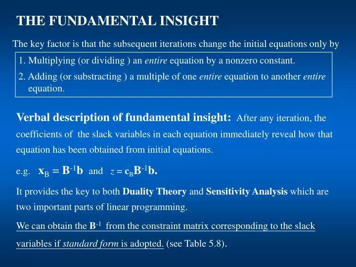
1. THE FUNDAMENTAL INSIGHT The key factor is that the subsequent iterations change the initial equations only by 1. Multiplying (or dividing ) an entire equation by a nonzero constant. 2. Adding (or substracting ) a multiple of one entire equation to another entire equation. Verbal description of fundamental insight: After any iteration, the coefficients of the slack variables in each equation immediately reveal how that equation has been obtained from initial equations. e.g. xB = B-1b and z = cBB-1b. It provides the key to both Duality Theory and Sensitivity Analysis which are two important parts of linear programming. We can obtain the B-1 from the constraint matrix corresponding to the slack variables if standard form is adopted. (see Table 5.8).

3. Iteration 0: . . . Iteration i:

4. Example. Iteration 1.

5. =

7. Iteration 2 =

8. Initial coefficients

9. The entire final tableau (except row 0) has been obtained from the initial tableau as z + (cBB-1A – c)x + cBB-1xs = cBB-1b

10. Mathematical Summary

12. S* = B-1 • Fundamental Insight • t* = t + y*T = [ y*A – c | y* | y*b ] • T* = S*T = [ S*A | S* | S*b ] Proof: Let unknown matrix be M such that T* = MT, [ A* | S* | b* ] = M [ A | I | b ] = [ MA | M | Mb ]  M = S* = B-1 Let unknown vector be v such that t* = t + vT, [ z* – c | y* | Z* ] = [ –c | 0 |0] + v [ A | I | b ] = [ –c + vA | v | vb ]  v = y* = cBB-1

13. Original variables Slack variables RHS z x xs z 1 cBB-1A - c cBB-1 cBB-1b xB 0 B-1A B-1 B-1b revised simplex method cBB-1A – c, cBB-1 determine pivot element (i.e. entering basic Variable and leaving Basic variable) only reduced costs for nonbasic variables iteration j iteration j+1

14. Original variables Slack variables RHS z x xs z 1 cBB-1A - c cBB-1 cBB-1b xB 0 B-1A B-1 B-1b revised simplex method determine pivot element (i.e. entering basic variable and leaving basic variable) Iteration j+1 iteration j (only calculate the necessary information)

15. Applications of Fundamental Insights: • Design the revised simplex method. In the revised simplex method, we may use B-1 and the initial tableau to calculate all the relevant numbers in the current tableau for every iteration. To calculate y* as y* = cBB-1. (2)Give the interpretation of the shadow prices. Let be the shadow prices. The fundamental insight reveals that optimal value z* is (look at the matrix form at the final iteration.)

16. The Overall Procedure

17. Original variables Slack variables RHS z x xs z 1 cBB-1A - c cBB-1 cBB-1b xB 0 B-1A B-1 B-1b

18. Original variables Slack variables RHS z x xs z 1 cBB-1A - c cBB-1 cBB-1b xB 0 B-1A B-1 B-1b revised simplex method determine pivot element (i.e. entering basic variable and leaving basic variable) cBB-1A – c, cBB-1 only reduced costs for nonbasic variables iteration j+1 iteration j

19. It can be expressed as

20. Example. ( initial basic variables which are slack variables.) x2   x4

21. [U1U3 ] Negative  not optimal To test the optimality, we calculate corresponding to basic variables

23. [U1U2] To test the optimality, we calculate Nonnegative  optimal

24. If we initiate the simplex procedure with a basis that is an identity matrix. Then, Iteration 0: B = I, B-1 = I; Iteration 1: B-1 = E1I-1 = E1; Iteration 2: B-1 = E2E1; . . . Iteration k: B-1 = EkEk-1 . . . E2E1; where Ei is the elementary matrix corresponding to the ith pivot operation. 1