Download
1 / 25
250 likes | 286 Vues
Explore the world of molecular modeling focusing on potential energy functions, molecular mechanics, force field parameters, and atomic charges in this detailed guide. Learn about various methods and software used for crystal structures and molecules.

E N D
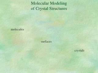
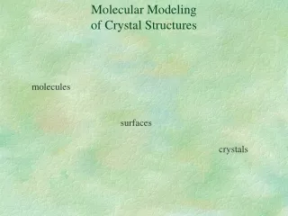
Molecular Modelingof Crystal Structures molecules surfaces crystals
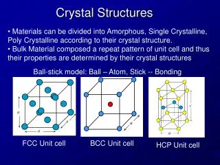
1. Potential energy functions QM ab initio: distribution of electrons over the system. Gaussian94, Gamess, ... Semi-empirical methods: pre-calculated values or neglect of some parts of the ab-initio calculation. MOPAC (mopac6, 7, 93, 2000) Empirical methods: observed/fitted values for interactions between atoms. Sybyl, Cerius2, Gromos, ...
Potential energy functions Differences: * Speed (as a function of system size) * Accuracy * Intended use (heat of fusion; conformational energies; transition states; vibrations/spectra; …) * Transferability / applicability * Availability / user interface
Potential energy functions Focus: Molecular Mechanics (MM) “Ball and Spring” model of molecules, based on simple equations giving U as function of atomic coordinates G = U + pV - TS H = U + pV EMM = U
EMM = Estretch + Ebend + Etorsion + Evdw + Ecoul + ... bonded non-bonded Molecular Mechanicssystem from atoms + bonds H H • stretching • bending • torsion H C C H H H
MM: interactions via bonds r Es = 1/2 ks(r-r0)2 … + C3(r-r0)3 + C4(r-r0)4 bond stretch E - True .. modeled via (r-r0)2 r0 r
C C C C E Force field parameters: bond lengths (Dreiding) Es = 1/2 ks(r-r0)2 Bond type r0 (Å) ks (kcal/mol.A2) C(sp3)--C(sp3) 1.53 700 C(sp3)--C(sp2) 1.43 700 C(sp2)--C(sp2) 1.33 1400 C(sp3)--H 1.09 700 kS=700: E=3 kcal ~ r=0.09Å
MM: interactions via bonds bending Eb = 1/2 kb(-0)2 E 0
E Force field parameters: bond angles (Dreiding) Angle type 0 (°) kb(kcal/mol.rad2) X--C(sp3)--X 109.471 100 X--O(sp3)--X 104.510 100 C O H E=3 kcal ~ =14°
C C Force field parameters: torsion angles (Dreiding) Etor = V1[1 - cos (-01) ] V2[1 - cos 2(-02)] V3[1 - cos 3(-03)] E V3 0 60 120 180
Force field parameters: torsion angles (Dreiding) C C torsion type n V (kcal/mol) 0 (°) X--C(sp3)--C(sp3)--X 3 1.0 180 X--C(sp2)--C(sp2)--X 2 22.5 0 C C
Non-bonded interactions: Van der Waals repulsive: ~r-10 attractive: ~r-6 E=D0[(r0/r)12-2(r0/r)6] (Lennard-Jones) E=D0{exp[a(r0/r)]-b(r0/r)6} (Buckingham; “exp-6”)
Non-bonded interactions: Coulomb (electrostatic) atomic partial charges: Eij=(qixqj)/(rij) atomic/molecular multipoles: E=ixj/Dr3 + - + - + +
additional energy terms in force fields * out-of-plane energy term * Hydrogen bond energy term
MM energy calculation EMM = Estretch + Ebend + Etorsion + Evdw + Ecoul + ... bonded non-bonded bonded non-bonded 1…2 1…3 1…4 1…4: scaled 1…5 1…6/7/8 5 1 2 3 4 8 6 7
Some available force fields FF software focus Gromos Gromos bio Charmm Charmm; Quanta bio Amber Amber bio Tripos Sybyl general Dreiding Cerius general Compass Cerius general CVFF Cerius general Glass2.01 Cerius ionic
Force field parameters:where do they come from? 1. Mimic physical properties of individual elements or atom types, producing a “physical” force field. Properties can be taken from experimental data, or ab-initio calculations. Examples: Dreiding, Compass. + outcome will be ‘reasonable’, predictable; extension to new systems relatively straightforward. - performance not very good.
Force field parameters:where do they come from? 2. Optimize all parameters with respect to a set of test data, producing a “consistent” force field. Test set can be chosen to represent the system under investigation. Examples: CFF, CVFF. + outcome often good for a particular type of systems, or a particular property (e.g. IR spectrum). - extension to new systems can be difficult; no direct link to ‘physical reality’
Force field parameters:where do they come from? 3. Apply common sense and look at what the neighbors do. Examples: Gromos. + does not waste time on FF parameterization; resonable results. - ?
Atomic charges Why? To include the effect of the charge distribution over the system. Some sp2 oxygens are more negative than others. How? Assign a small charge to each atom. Caveat: interaction with other force field parameters (e.g. VdW).
Atomic charges • What is the atomic charge? • * Based on atomic electronegativity, optimized for a given FF. • example: Gasteiger charges. • Based on atomic electronegativity and the resulting electrical field. • example: Charge Equilibrium charges (QEq). • * Based on the electronic distribution calculated by QM. • example: Mulliken charges. • * Based on the electrostatic potential near the molecule, • calculated by a non-empirical method (or determined experimentally). • examples: Chelp, ChelpG, RESP.
Atomic charges Properties and features of different charge schemes: * Depends on molecular conformation? * Easy (=quick) to calculate? * Performance in combination with force field? Known-to-be-good combinations: Tripos -- Gasteiger Dreiding -- ESP Compass -- Compass
Atomic charges:charges fitted to the ElectroStatic Potential (ESP) mechanism: Coulomb interactions result from the electrostatic potential around a molecule. + + + + - - + H - - - H+ - O - - - - H + + + + +
H sample point O H Atomic charges:charges fitted to the ElectroStatic Potential (ESP) molecule QM wave function electron density sample true ESP mathematical fit for each sample point: atomsq/r= ESPQM * atomic q as variables atomic charges that reproduce the true ESP
Atomic charges:charges fitted to the ElectroStatic Potential (ESP) Properties and features of different fittingschemes: * Number of sample points. * Position of sample points. * Additional restraints (e.g. all qH in CH3 equal). * Fitting to multiple conformations. Known-to-be-good fitting schemes: ChelpG RESP