Download
1 / 30
310 likes | 623 Vues
The Analysis of Volatility. Historical Volatility. Volatility Estimation (MLE, EWMA, GARCH...). Maximum Likelihood Estimation. Implied Volatility. Smiles, smirks, and explanations. In the Black-Scholes formula, volatility is the only variable that is not directly observable in the market.

E N D
The Analysis of Volatility Primbs, MS&E 345, Spring 2002
Historical Volatility Volatility Estimation (MLE, EWMA, GARCH...) Maximum Likelihood Estimation Implied Volatility Smiles, smirks, and explanations Primbs, MS&E 345, Spring 2002
In the Black-Scholes formula, volatility is the only variable that is not directly observable in the market. Therefore, we must estimate volatility in some way. Primbs, MS&E 345, Spring 2002
Change to log coordinates and discretize: Then, an unbiased estimate of the variance using the m most recent observations is where A Standard Volatility Estimate: (I am following [Hull, 2000] now) Primbs, MS&E 345, Spring 2002
Unbiased estimate means Max likelihood estimator Minimum mean squared error estimator Note: If m is large, it doesn’t matter which one you use... Primbs, MS&E 345, Spring 2002
For simplicity, people often set and use: is an estimate of the mean return over the sampling period. In the future, I will set as well. Note: Why is this okay? It is very small over small time periods, and this assumption has very little effect on the estimates. Primbs, MS&E 345, Spring 2002
The estimate gives equal weight to each ui. Alternatively, we can use a scheme that weights recent data more: where Weighting Schemes Furthermore, I will allow for the volatility to change over time. So sn2 will denotes the volatility at day n. Primbs, MS&E 345, Spring 2002
Assume there is a long run average volatility, V. where Weighting Schemes An Extension This is known as an ARCH(m) model ARCH stands for Auto-Regressive Conditional Heteroscedasticity. Primbs, MS&E 345, Spring 2002
y regression: y=ax+b+e x x x x e is the error. x x x x x x x x x Homoscedastic and Heteroscedastic If the variance of the error e is constant, it is called homoscedastic. However, if the error varies with x, it is said to be heteroscedastic. Primbs, MS&E 345, Spring 2002
Exponentially Weighted Moving Average (EWMA): weights die away exponentially Weighting Schemes Primbs, MS&E 345, Spring 2002
GARCH(1,1) Model Generalized Auto-Regressive Conditional Heteroscedasticity where The (1,1) indicates that it depends on Weighting Schemes You can also have GARCH(p,q) models which depend on the p most recent observations of u2 and the q most recent estimates of s2. Primbs, MS&E 345, Spring 2002
Historical Volatility Volatility Estimation (MLE, EWMA, GARCH...) Maximum Likelihood Estimation Implied Volatility Smiles, smirks, and explanations Primbs, MS&E 345, Spring 2002
That is, we solve: where f is the conditional density of observing the data given values of the parameters. How do you estimate the parameters in these models? One common technique is Maximum Likelihood Methods: Idea: Given data, you choose the parameters in the model the maximize the probability that you would have observed that data. Primbs, MS&E 345, Spring 2002
Let Maximum Likelihood Methods: Example: Estimate the variance of a normal distribution from samples: Given u1,...,um. Primbs, MS&E 345, Spring 2002
where K1, and K2 are some constants. To maximize, differentiate wrt v and set equal to zero: Maximum Likelihood Methods: Example: It is usually easier to maximize the log of f(u|v). Primbs, MS&E 345, Spring 2002
where We don’t have any nice, neat solution in this case. You have to solve it numerically... Maximum Likelihood Methods: We can use a similar approach for a GARCH model: The problem is to maximize this over w, a, and b. Primbs, MS&E 345, Spring 2002
Historical Volatility Volatility Estimation (MLE, EWMA, GARCH...) Maximum Likelihood Estimation Implied Volatility Smiles, smirks, and explanations Primbs, MS&E 345, Spring 2002
Denote the Black-Scholes formula by: The value of s that satisfies: is known as the implied volatility Implied Volatility: Let cm be the market price of a European call option. This can be thought of as the estimate of volatility that the “market” is using to price the option. Primbs, MS&E 345, Spring 2002
Implied Volatility smile smirk K/S0 The Implied Volatility Smile and Smirk Market prices of options tend to exhibit an “implied volatility smile” or an “implied volatility smirk”. Primbs, MS&E 345, Spring 2002
Where does the volatility smile/smirk come from? Heavy Tail return distributions Crash phobia (Rubenstein says it emerged after the 87 crash.) Leverage: (as the price falls, leverage increases) Probably many other explanations... Primbs, MS&E 345, Spring 2002
Why might return distributions have heavy tails? Heavy Tails Stochastic Volatility Jump diffusion models Risk management strategies and feedback effects Primbs, MS&E 345, Spring 2002
Out of the money call: Call option strike K More probability under heavy tails At the money call: Probability balances here and here Call option strike K How do heavy tails cause a smile? This option is worth more This option is not necessarily worth more Primbs, MS&E 345, Spring 2002
Mean Variance Skewness Kurtosis Important Parameters of a distribution: Gaussian~N(0,1) 0 1 0 3 Primbs, MS&E 345, Spring 2002
Mean Variance Skewness Kurtosis Red (Gaussian) 0 1 0 3 Blue 0 1 -0.5 3 Skewness tilts the distribution on one side. Primbs, MS&E 345, Spring 2002
Mean Variance Skewness Kurtosis Red (Gaussian) 0 1 0 3 Blue 0 1 0 5 Large kurtosis creates heavy tails (leptokurtic) Primbs, MS&E 345, Spring 2002
Empirical Return Distribution Mean Variance Skewness Kurtosis 0.0007 0.0089 -0.3923 3.8207 (Data from the Chicago Mercantile Exchange) (Courtesy of Y. Yamada) Primbs, MS&E 345, Spring 2002
Volatility Smiles and Smirks 10 days to maturity Mean Square Optimal Hedge Pricing (Courtesy of Y. Yamada) Primbs, MS&E 345, Spring 2002
Volatility Smiles and Smirks 20 days to maturity Mean Square Optimal Hedge Pricing (Courtesy of Y. Yamada) Primbs, MS&E 345, Spring 2002
Volatility Smiles and Smirks 40 days to maturity Mean Square Optimal Hedge Pricing (Courtesy of Y. Yamada) Primbs, MS&E 345, Spring 2002
Volatility Smiles and Smirks 80 days to maturity Mean Square Optimal Hedge Pricing (Courtesy of Y. Yamada) Primbs, MS&E 345, Spring 2002