Download

1 / 20
230 likes | 542 Vues
Elements of kinetic theory. Introduction Phase space density Equations of motion Average distribution function Boltzmann-Vlasov equation Velocity distribution functions Moments and fluid variables The kinetic plasma temperature. Introduction.

E N D
Elements of kinetic theory • Introduction • Phase space density • Equations of motion • Average distribution function • Boltzmann-Vlasov equation • Velocity distribution functions • Moments and fluid variables • The kinetic plasma temperature
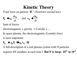
Introduction Kinetic theory describes the plasma statistically, i.e. the collective behaviour of the various particles under the influence of their self-generated electromagnetic fields. • Collective behaviour and complexity arises from: • Many particles (species: electrons, protons, heavy ions) • Long-range self-consistent fields, B(x,t) and E(x,t) • Fields as averages over the microscopic fields generated by all particles together • Strong mutual interactions between fields and particles may lead to nonlinearities
Phase space Six-dimensional phase space with coordinates axes x and v and volume element dxdv Many particles (i=1, N) having time-dependent position xi(t) and velocity vi(t). The particle path at subsequent times (t1,.., t5) is a curve in phase (see illustration right figure).
Phase space density For each individual particle (index i) we may define the exact density in phase space through sharp three-dimensional delta functions ( (x) = (x) (y) (z) ) as follows: The multi-particle density is simply obtained by summation over all particles (of all components). The geometrical content is that the phase space volume occupied consists of the sum of all individual phase space volume elements. Since particles are subject to the action of forces (different for different particles), the total phase space volume will deform but remain constant (particle number conservation).
Equation of motion with electromagnetic forces Deformation of dxdv due to microscopic force. (3-d: dv=d3v=dvxdvydvz) The instantaneous velocity is vi=dxi(t)/dt, with the total derivate with respect to time. Denoting the microscopic field by index m, the equation of motion reads:
Maxwell equations Ampère, Faraday, Gauß Microscopic electromagnetic fields Microscopic charge and current densities
Klimontovich equation If no particles are lost from or added to the plasma the exact phase space density is conserved. Thus the total time derivative vanishes, and is in 6-d phase space given after the chain rule of differentiation as follows: This still describes the plasma state fully at all times.
Boltzmann equation We now define an ensemble averaged phase space density, the distribution function, through the decomposition: with vanishing fluctuations: = 0. Similarly, the microscopic field is decomposed: Inserting these decompositions into the Klimontovich equation yields after ensemble averaging the Boltzmann equation.
Models for the collision terms The second-order term on the right of the Boltzmann equation contains all correlations between fields and particles, due to collisions and (wave-) fluctuation-particle interactions, and is notoriously difficult to evaluate. Concerning neutral-ion collisions a simple relaxation approach is sometimes applied, with fn being the velocity distribution function (VDF) of the neutrals, and n is their collision frequency: Collisions (Landau or Fokker-Planck) and wave-particle interactions can often be described as a diffusion process:
Vlasov equation Since most space plasmas are collisionless, we neglect the right-hand side in the Boltzmann equation and thus obtain the simplest kinetic equation named after Vlasov: This equation expresses phase space density conservation (Liouville theorem) visualised in the left figure. A volume element evolves under the Lorentz force like in an imcompressible fluid and remains constant as the number of particles contained in it. The Vlasov equation is still highly nonlinear via closure with Maxwell‘s equations.
Maxwellian velocity distribution function The general equilibrium VDF in a uniform thermal plasma is the Maxwellian (Gaussian) distribution. The average velocity spread (variance) is, <v> = (2kBT/m)1/2, and the mean drift velocity, v0.
Anisotropic model velocity distributions The most common anisotropic VDF in a uniform thermal plasma is the bi-Maxwellian distribution. Left figure shows a sketch of it with T > T .
Loss-cone model distribution function Here and are parameters to fit the loss cone. =0 gives an empty loss cone, and =1 reproduces a simple Maxwellian. allows to change the slope of f inside the loss cone.
Kappa and power-law distribution function Differential particle flux function, J(W) ~ v2 f(v). Here is a shape parameter. If >> 1, the distribution approaches a Maxwellian, = 2 is a Lorentzian, and for small > 2 the VDF has a power-law tail in proportion to (W0/W)-, with the average thermal energy W0=kBT (1-3/2).
Measured solar wind proton velocity distributions • Temperature anisotropies • Ion beams • Plasma instabilities • Interplanetary heating Plasma measurements made at 10 s resolution ( > 0.29 AU from the Sun) Marsch et al., JGR, 87, 52, 1982 Helios
Measured solar wind electrons Helios Sun ne = 3 -10 cm-3 • Non-Maxwellian • Heat flux tail Pilipp et al., JGR, 92, 1075, 1987
Velocity moments I The microsopic distribution depends on v, x, and t. The macroscopic physical parameters, like density or temperature, depend only on x and t and thus are obtained by integration over the entire velocity space as so-called moments. The i-th moment is the following integral: Where vi = vv...v (i-fold) denotes an i-fold dyadic product, i.e. a tensor of rank i.
Velocity moments II The number density is defined as 0-th order moment: The bulk flow velocity is defined as 1-st order moment: The pressure tensor is defined as the fluctuation of the velocities of the ensemble from the mean velocity, i.e. as the 2-nd order moment:
Velocity moments III The trace-less parts of the pressure tensor P correspond to the stresses in the plasma. The heat flux tensor is used to describe the multi-directional flow of internal energy and defined as 3-rd order moment: More relevant to decribe deviations from thermal equilibrium is the trace of Q, the heat flux vector, q, that is defined as:
Concept of temperature The isotropic scalar pressure is defined as the trace of P, i.e.p = 1/2 Pii, which leads through the ideal gas law, p = nkBT, to the kinetic temperature defined as 2-nd moment: This temperature can formally be calculated for any VDF and thus is not necessarily identical with the thermodynamic temperature. To demonstrate its meaning, calculate the kinetic temperature for the Maxwellian at rest: Note that by integration, with the volume element d3v = 4v2dv, one finds (exercise!) that