Download
1 / 37
400 likes | 790 Vues
Demography, Metapopulations, and PVA. Overview. Basic population ecology Metapopulations Stochasticity PVA. What is a population?. What are models anyway and what are they for?. “A formalization of your assumptions about a systemâ€- Charles Hall

E N D
Overview • Basic population ecology • Metapopulations • Stochasticity • PVA
What are models anyway and what are they for? • “A formalization of your assumptions about a system”- Charles Hall • Abstractions of nature. A hypothesized set of rules governing a system • Used for?
What is demography? The study of the size, composition and trajectory of populations through time
Can we influence these factors and, thereby, affect the fate of the population? Why does demographyplay a central role in Conservation Biology? • Species extinction is a population level process • We wish to know • Is a population likely to go extinct? • What are key factors in determining a population’s fate?
How does demography relate to the rest of this class? • Demographic variables are key indicators of the status of biodiversity • ESA: lists species “in danger of extinction” • IUCN criteria: • Eg. Critically endangered: Expected 80% decline or 50% probability of extinction in next 10 years or 3 generations.
2008 IUCN Red List • Biggest revision since 1996 • 44,838 spp. listed • 16,928 threatened • ¼ mammals listed as threatened • Tasmanian devil moved from ‘least concern’ to ‘endangered’ • Rameshwaram parachute spider listed as critically endangered • Holdridge's toad listed as extinct • La Palma giant lizard rediscovered, moved to critically endangered
Simple Population Models • Exponential Growth • “There is no conservation problem that could not be solved, indeed turned into a pest problem, by a little exponential growth.” —Hal Caswell • Nt = N0ert r = intrinsic rate of increase • dN/dt = rN = per capita rate of increase • r=0 stable • r>0 growth • r<0 decline
Simple Population Models • Geometric Growth (Exponential growth with discrete intervals) Nt = N0t = finite rate of increase Or Nt+1 = Ntt = er = Nt /N0
Geometric Growth • Example N0 =50 Nt =100 =100/50 =2 • =1 stable • >1 growth • <1 decline
Modeling Growth • Simple Logistic Growth • A simple model for density dependence • dN/dt = rN(1-N/K) K=carrying capacity K
METAPOPULATIONS • Aggregation of subpopulations (demes), at least some of which are extinction prone and between which there is dispersal (ie. colonization)
METAPOPULATIONS Why is the issue important in Conservation Biology? http://www.rr.ualberta.ca/courses/renr575/fragmentationphotos.htm Anthropogenic changes create metapopulation-type systems. Understanding the demographic processes within these systems is critical in predicting species decline or extinction
Theory of island biogeography (MacArthur and Wilson 1967) http://www.algebralab.org/practice/practice.aspx?file=Reading_IslandBiogeography.xml
METAPOPULATIONS • Classic Levins Model (1969) • Many discrete patches of () same size with () same extinction probability • Extinction probability () independent in each patch (asychronous dynamics) • Spatial pattern of patches not important (dispersal distances sufficiently large) • Patches are either occupied or not (no internal dynamics)
Levine’s Equation dP/dt=cP(1-P)-eP • P=proportion of patches that are occupied • dP/dt=colonization rate – extinction rate • c = colonization rate • e = extinction rate • Colonization (c) = [(# vacant sites occupiedt=1)/(# vacant sitest=0)] • Extinction (e) = [(# sites occupied site that went extinctt=1)/(# occupied sitest=0)]
METAPOPULATIONS • What proportion are occupied at equilibrium? Peq=1-e/c
METAPOPULATIONS • What can we learn from this equation Peq=1-e/c ? • If e > c, population will go extinct • If we assume that increased patch size correlates with low e, and patch isolation w/ low c: Distant Low Probability of Metapopulation Persistence Patch Spacing High Near Small Large Patch Size
5 Conservation Messages from Metapopulation Biology (Hanski 1997) • Unoccupied patches can be important • Appearances can be deceiving. Preserving the landscape as is may not be enough b/c of extinction debts • At least 10 patches are needed (based on stochastic models- Thomas and Hanski 1997) • Patch spacing is a compromise • Variance in habitat quality is beneficial
What is a stochastic model? • A model in which some parameters are allowed to fluctuate according to a random function
Stochasticity Average = 1.1… we would expect growth However… σ = 0.1 <1 >1
w/ demo. stoch. deterministic GRIZZLY BEAR PROJECTION W/ DEMOGRAPHIC STOCHASTICITY (Shaffer 1981, 1983)
N(0)=47 N(0)=5 The importance of demographic stochasticity decreases as populations gets larger (Shaffer 1981, 1983)
Population Viability Analysis (PVA) • Morris and Doak (2002) • Use of quantitative methods to predict the likely future status of a population • ‘Future status’- likelihood that the population will be above some minimum size at a given future time • Can be deterministic but stochastic models are most accepted
The extinction vortex (Soule and Mills 1998; Frankham et al. 2002)
Population Viability Analysis (PVA) • ‘Quasi-extinction threshold’ (and related outputs) • Time • P(E) vs. P(P) • Conclusions are probabilistic (stochastic) • PVA is used in endangered species recovery plans and for IUCN rankings • CBSG- PVHAs
Sensitivity & Elasticity Analysis • Which parameters in the model are most influential on growth rate (), N, or some aspect of the population • Perturb each parameter (one at a time) a small amount while holding all other constant and observe the impact on, say,
Sensitivity & Elasticity Analysis • Sensitivity of to change in a specific parameter (eg, survival of first year) is the change in per unit change in that parameter. ABSOLUTE CHANGE • Elasticity of is the proportional change of (eg 50%) resulting from a proportional change in one of the matrix elements. RELATIVE CHANGE
Why do Sensitivity & Elasticity Analysis? • Identify life stages to focus management upon (e.g. endangered species, threatening exotics) • Focus field studies • Note, some sensitive rates may not vary (e.g. Albatrosses lay one egg)
SENSITIVITY ANALYSIS FOR MODELS OF POPULATION VIABILITY (helmeted honeyeater Lichenostomus melanops cassidix) McCarthy, Burgman and Ferson, Biological Conservation 1995)