Download
1 / 54
620 likes | 1.17k Vues
Introduction to Graph Theory. Presented by Mushfiqur Rouf (100505056). Graph Theory - History. Leonhard Euler's paper on “ Seven Bridges of Königsberg” , published in 1736. . Famous problems. “The traveling salesman problem”

E N D
Introduction to Graph Theory Presented by Mushfiqur Rouf (100505056)
Graph Theory - History Leonhard Euler's paper on “Seven Bridges of Königsberg” , published in 1736.
Famous problems • “The traveling salesman problem” • A traveling salesman is to visit a number of cities; how to plan the trip so every city is visited once and just once and the whole trip is as short as possible ?
Famous problems In 1852 Francis Guthrie posed the “four color problem” which asks if it is possible to color, using only four colors, any map of countries in such a way as to prevent two bordering countries from having the same color. This problem, which was only solved a century later in 1976 by Kenneth Appel and Wolfgang Haken, can be considered the birth of graph theory.
Examples • Cost of wiring electronic components • Shortest route between two cities. • Shortest distance between all pairs of cities in a road atlas. • Matching / Resource Allocation • Task scheduling • Visibility / Coverage
Examples • Flow of material • liquid flowing through pipes • current through electrical networks • information through communication networks • parts through an assembly line • In Operating systems to model resource handling (deadlock problems) • In compilers for parsing and optimizing the code.
What is a Graph? • Informally a graph is a set of nodes joined by a set of lines or arrows. 1 2 3 1 3 2 4 4 5 6 5 6
Definition: Graph • G is an ordered triple G:=(V, E, f) • V is a set of nodes, points, or vertices. • E is a set, whose elements are known as edges or lines. • f is a function • maps each element of E • to an unordered pair of vertices in V.
Definitions • Vertex • Basic Element • Drawn as a node or a dot. • Vertex set of G is usually denoted by V(G), or V • Edge • A set of two elements • Drawn as a line connecting two vertices, called end vertices, or endpoints. • The edge set of G is usually denoted by E(G), or E.
Example • V:={1,2,3,4,5,6} • E:={{1,2},{1,5},{2,3},{2,5},{3,4},{4,5},{4,6}}
Simple Graphs Simple graphs are graphs without multiple edges or self-loops.
A B C Cycle D 1 F E 3 2 Unreachable 4 5 6 Cycle Path • A path is a sequence of vertices such that there is an edge from each vertex to its successor. • A path is simple if each vertex is distinct. Simple path from 1 to 5 = [ 1, 2, 4, 5 ] Our text’s alternates the verticesand edges. If there is path p from u to v then we say v is reachable from u via p.
A B C Cycle D 1 F E 3 2 Unreachable 4 5 6 Cycle Cycle • A path from a vertex to itself is called a cycle. • A graph is called cyclic if it contains a cycle; • otherwise it is called acyclic
Connectivity • is connected if • you can get from any node to any other by following a sequence of edges OR • any two nodes are connected by a path. • A directed graph is strongly connected if there is a directed path from any node to any other node.
Sparse/Dense • A graph is sparse if | E | | V | • A graph is dense if | E | | V |2.
2 1.2 1 3 1 2 3 2 .2 1.5 5 .5 3 .3 1 4 5 6 4 5 6 .5 A weighted graph • is a graph for which each edge has an associated weight, usually given by a weight functionw: E R.
Directed Graph (digraph) • Edges have directions • An edge is an ordered pair of nodes
Bipartitegraph • V can be partitioned into 2 sets V1 and V2such that (u,v)E implies • either uV1 and vV2 • OR vV1 and uV2.
Special Types • Empty Graph / Edgeless graph • No edge • Null graph • No nodes • Obviously no edge
Complete Graph • Denoted Kn • Every pair of vertices are adjacent • Has n(n-1) edges
Complete Bipartite Graph • Bipartite Variation of Complete Graph • Every node of one set is connected to every other node on the other set
Planar Graph • Can be drawn on a plane such that no two edges intersect • K4 is the largest complete graph that is planar
Dual Graph • Faces are considered as nodes • Edges denote face adjacency • Dual of dual is the original graph
Tree • Connected Acyclic Graph • Two nodes have exactly one path between them
Generalization: Hypergraph • Generalization of a graph, • edges can connect any number of vertices. • Formally, an hypergraph is a pair (X,E) where • X is a set of elements, called nodes or vertices, and • E is a set of subsets of X, called hyperedges. • Hyperedges are arbitrary sets of nodes, • contain an arbitrary number of nodes.
A B C D F E The degree of B is 2. Degree • Number of edges incident on a node
1 2 4 5 The in degree of 2 is 2 andthe out degree of 2 is 3. Degree (Directed Graphs) • In degree: Number of edges entering • Out degree: Number of edges leaving • Degree = indegree + outdegree
Degree: Simple Facts • If G is a digraph with m edges, then indeg(v) = outdeg(v) = m = |E | • If G is a graph with m edges, then deg(v) = 2m= 2 |E | • Number of Odd degree Nodes is even
Subgraph • Vertex and edge sets are subsets of those of G • a supergraph of a graph G is a graph that contains G as a subgraph. • A graph G contains another graph H if some subgraph of G • is H or • is isomorphic to H. • H is a proper subgraph if H!=G
Spanning subgraph • Subgraph H has the same vertex set as G. • Possibly not all the edges • “H spans G”.
Induced Subgraph • For any pair of vertices x and y of H, xy is an edge of H if and only if xy is an edge of G. • H has the most edges that appear in G over the same vertex set.
Induced Subgraph (2) • If H is chosen based on a vertex subset S of V(G), then H can be written as G[S] • “induced by S” • A graph that does not contain H as an induced subgraph is said to be H-free
Component • Maximum Connected sub graph
Isomorphism • Bijection, i.e., a one-to-one mapping: f : V(G) -> V(H) u and v from G are adjacent if and only if f(u) and f(v) are adjacent in H. • If an isomorphism can be constructed between two graphs, then we say those graphs are isomorphic.
Isomorphism Problem • Determining whether two graphs are isomorphic • Although these graphs look very different, they are isomorphic; one isomorphism between them is f(a) = 1 f(b) = 6 f(c) = 8 f(d) = 3 f(g) = 5 f(h) = 2 f(i) = 4 f(j) = 7
Graph ADT • In computer science, a graph is an abstract data type (ADT) • that consists of • a set of nodes and • a set of edges • establish relationships (connections) between the nodes. • The graph ADT follows directly from the graph concept from mathematics.
Representation (Matrix) • Incidence Matrix • E x V • [edge, vertex] contains the edge's data • Adjacency Matrix • V x V • Boolean values (adjacent or not) • Or Edge Weights
Representation (List) • Edge List • pairs (ordered if directed) of vertices • Optionally weight and other data • Adjacency List
Implementation of a Graph. • Adjacency-list representation • an array of |V | lists, one for each vertex in V. • For each uV , ADJ [ u ] points to all its adjacent vertices.
Adjacency-list representation for a directed graph. 2 5 1 1 2 2 5 3 4 3 3 4 5 4 4 5 5 5 Variation: Can keep a second list of edges coming into a vertex.
Adjacency lists • Advantage: • Saves space for sparse graphs. Most graphs are sparse. • Traverse all the edges that start at v, in (degree(v)) • Disadvantage: • Check for existence of an edge (v, u) in worst case time (degree(v))
Adjacency List • Storage • For a directed graph the number of items are(out-degree (v)) = | E | So we need ( V + E ) • For undirected graph the number of items are(degree (v)) = 2 | E | Also ( V + E ) • Easy to modify to handle weighted graphs. How? v V v V
1 2 3 4 5 1 2 3 0 1 0 0 1 1 2 3 4 5 1 0 1 1 1 5 4 0 1 0 1 0 0 1 1 0 1 1 1 0 1 0 Adjacency matrix representation • |V | x |V | matrix A = ( aij ) such that aij = 1 if (i, j ) E and 0 otherwise.We arbitrarily uniquely assign the numbers 1, 2, . . . , | V | to each vertex.
Adjacency Matrix Representation for a Directed Graph 1 2 3 4 5 0 1 0 0 1 1 2 3 4 5 1 2 0 0 1 1 1 0 0 0 1 0 3 0 0 0 0 1 5 4 0 0 0 0 0
Adjacency Matrix Representation • Advantage: • Saves space for: • Dense graphs. • Small unweighted graphs using 1 bit per edge. • Check for existence of an edge in (1) • Disadvantage: • Traverse all the edges that start at v, in (|V|)
Adjacency Matrix Representation • Storage • ( | V |2) ( We usually just write, (V2) ) • For undirected graphs you can save storage (only 1/2(V2)) by noticing the adjacency matrix of an undirected graph is symmetric. How? • Easy to handle weighted graphs. How?