Differences Between Everyday Tables and Database Tables
Learn the differences between everyday tables and database tables, use XML to describe table metadata, understand entities and attributes in database design, utilize database operations, express queries using Query By Example, and differentiate between physical and logical databases.


Differences Between Everyday Tables and Database Tables
E N D
Presentation Transcript
Learning Objectives • Explain the differences between everyday tables and database tables • Use XML to describe the metadata for a table of information, and classify the uses of the tags as identification, affinity, or collection • Understand how the concepts of entities and attributes are used to design a database table • Use the six database operations: Select, Project, Union, Difference, Product, and Join • Express a query using Query By Example • Describe the differences between physical and logical databases
Differences Between Tables and Databases • When we think of databases, we think of tables of information: • iTunes show the title, artist, running time on a row • Your car’s information is one line in the state’s database of automobile registrations • The U.S. is a row in the demography table for the World’s listing of country name, population, etc.
Comparing Tables • These images show how the row of data is described using tags
The Database’s Advantage • Metadata is the key advantage of databases over other approaches to recording data as tables • enables content search • Two most important roles in defining metadata • Identify the type of data: each different type of value is given a unique tag • Define the affinity of the data: Tags enclose all data that is logically related
XML:A Language for Metadata Tags • XML stands for the Extensible Markup Language • It is a tagging scheme • What makes XML easy and intuitive is that there are no standard tags to learn • Tags are created as needed • This trait makes XML a self-describing language
XML:A Language for Metadata Tags • There are a couple of rules: • Always match tags • Basically anything goes • XML works well with browsers and Web-based applications • XML must be written with a text editor to avoid unintentionally including the word processor’s tags (see Chapter 4)
XML • As with HTML, the tag and its companion closing tag surround the data • XML tag names cannot contain spaces • Both UPPERCASE and lowercase are allowed • XML is case sensitive • Like HTML, XML doesn’t care about white space between tags
XML Example • Scenario: • Create a database for the Windward Islands archipelago in the South Pacific • Plan what information will be stored • Develop those tags: <archipelago> <island> <iName> Tahiti </iName> <area>1048</area> </island> ⁞ </archipelago> Affinity role
XML <?xml version = "1.0" encoding="UTF-8" ?> • This required line is added at the beginning of the file • Note the question marks. • This line identifies the file as containing XML data representations • The file also has standard UTF-8 encoded characters
Expanding the Use of XML • To create a database of the two similar items (in this chapter, archipelagos), put both sets of information in the file • As long as the two sets use the same tags for the common information, they can be combined • Extra data is allowed and additional tags can be created (<a_name> to identify which archipelago is being used)
Expanding the Use of XML • Group sets of information by surrounding them with tags • These tags are the root elements of the XML database • A root element is the tag that encloses all content of the XML file • In Figure 15.1 the <archipelago> tag was the root element
Attributes in XML • HTML tags can have attributes to give additional information • Tags of XML also have attributes • They have a similar form • Must always be set inside simple quotation marks • Tag attribute values can be enclosed either in paired single or paired double quotes
Attributes in XML • Writing tag attributes is easy enough • The rules for using quotes are straightforward • Use attributes for additional metadata, not for actual content
Effective Design with XML Tags • XML is a flexible way to encode metadata • Identification Rule: Label Data with Tags Consistently • You choose the tags, but once you’ve decided you must always surround that kind of data with that tag • Keeps data together
Effective Design with XML Tags • Affinity Rule: Group Data Referencing an Entity • Enclose in a pair of tags all tagged data referring to the same thing • Grouping it keeps it all together, but it also makes an association of the tagged data items as being related to each other
Effective Design with XML Tags • Collection Rule: Group Instances • When you have several instances of the same kind of data, enclose them in tags • Keeps them together and implies that they are instances of the same type
The XML Tree • The rules for producing XML encodings of information produce hierarchical descriptions • Can be thought of as trees • The hierarchy is a consequence of how the tags enclose one another and the data
Tables and Entities • Lets set aside the tagging and XML and focus on database tables • The XML tree on the next slide shows the root element to the left and the leaves (content) to the right
Database Tables • Any group of things with common characteristics that specifically identify each one can be formed into a database table • Contains a set of things with common attributes
Database Vocabulary • Entities: rows of the database table • Attribute Name: column heading • Entity Instance: value in a row • Table Instance: whole table
What to Notice • Rows are all different • Two rows can have the same value for some attributes, but not all • Even when we don’t know the data for an attribute value it is still a characteristic • The rows can be in any order • The columns can be in any order
What to Notice • Rearranging the rows or columns will result in the same table • If we add (or remove) rows, or change a value we create a new table instance
Properties of Entities • A database table can be empty • It is a table with no rows • An entity is anything defined by a specific set of attributes • A table exists with a name and column headings • Once entity instances have been specified, there will be rows • Among the instances of any table is the “empty instance”
Every Entity Must Be Different • Amoebas are not entities, because they have no characteristics that allow us to tell them apart • One-celled animals are entities • In cases where it is difficult to process the information specifically identifying an entity, we might select an alternate encoding • Entities are the data of databases
Relational Database Tables • Tables are technically called relations, but we’ll continue to call them database tables • The rows must always be different, even after adding rows • Be sure the table has all of the attributes (columns) needed to tell the entities apart • You can always add a sequence number to guarantee that every row is different
Keys • By itself, repeated data in a column is not a problem • We are interested in columns in which all of the entries are always different, because they can be used to look up data • such a column is called a candidate key • doesn't have to be just one column (it can be multiple columns together)
Keys • Primary Key: candidate key that the computer and user agree will be used to locate entries during database operations
A Database Table’s Metadata • It is possible to succinctly describe a database table with a database scheme or database schema • Attributes are listed, one per row • For each attribute, the user specifies its data type and whether or not it is the primary key • It is also customary to include a brief description • The database scheme is the database table’s metadata PLAN
Computing with Tables • To get information from database tables, we write a query describing what we want • Query: command that tells the database system how to manipulate its tables to compute the answer • the answer will be in the form of another database table • We need to know 6 operations
Project Operation • Project (pronounced prōJECT) picks out and arranges columns from one database table to create a new, possibly “narrower”, table
Select Operation • The Select operation picks out rows according to specified criterion
Cross-Product Operation • Combines two tables in a process like multiplication • For each row in the first table, we make a new row by appending a row from the second table • All combinations are in the result
Cross-Product Operation • Because we pair all rows, a table with m rows crossed with a table with n rows will produce a table with m*n rows • Using cross-product with other table operations is powerful • Often follow with a select to choose wanted entities • Then a project to narrow to wanted attributes
Union Operation • Combines two tables with compatible attributes (columns) • The result has rows from both tables • For any rows that are in both tables, only one copy is included in the result
Difference Operation • The opposite of the Union operation • D1 – D2 contains the rows of the D1 table that are not also in the D2 table
Join Operation • Join is a combination of a Cross-Product, followed by a Select operation • Takes two database tables, and an attribute from each one (D1.a1 and D2.a2)
Join Operation • Join crosses the two tables and then uses Select to find those rows of the cross in which the two attributes match D1.a1 = D2.a2 • Puts tables together while matching up related data