Chapter 4 Random Processes
Chapter 4 Random Processes. 4.2 Random processes : Basic concepts 4.2.1Description of Random Process. Def : for each S , we assign a time function depicted by X (t, ) or . (i.e. we assign a function X (t, ) to every outcome )

Chapter 4 Random Processes
E N D
Presentation Transcript
Chapter 4 Random Processes
4.2 Random processes : Basic concepts 4.2.1Description of Random Process Def : for each S , we assign a time function depicted by X (t, ) or . (i.e. we assign a function X (t, ) to every outcome ) The family { ( ) : } forms a stochastic process Domain of , D ( ) = --- sample space Domain of t , D ( t ) = I --- A set of real number R
1 2 3 4 the meaning of X(t) : A family (an ensemble ) : t and are variables A single time function : t is a variable . is fixed . A random variable : t is a fixed , is a variable . A number : t , are fixed . , ...... state space
Classification of a RP : depend upon three quantities : • The state spaces, • the index time parameter, • and the statistical dependences. • state space : ( The collection of every value ) • Discrete-state process (chain) • Continuous-state process • index ( time ) parameter : • discrete-time process , , X[n] • continuous-time process , , X(t) • statistical dependence (e.g. sss , wss , independence process , ... , etc .)
Def. 4.2.1 A complete statistical description of a R.P. X(t) is known if for any integer n and any choice of ( , ,..., ) , the joint p.d.f. of is given and denoted by Def. 4.2.2 A process X(t) is described by its Mth order statistics if for all nM and all ( , ,..., ) ,the joint p.d.f. of is given . Note : M=2 : Second – order statistics
Example 4.2.3 A R.P. X(t) = , is a R.V. uniformly distributed on [0 , 2 ]
Example 4.2.4 X(t) = X, X is a r.v. uniformly distributed on [-1,1]
Example 4.2.5 A complete statistical description X(t) , t>0 for any n and any ( , ,..., ) , is a jointly Gaussian distribution with mean 0 and covariance matrix described by
4.2.2 Statistical Averages Def: Mean of R.P. X(t) : (a determinate function of t )
Example 4.2.6. The mean of R.P. in Example 4.2.3 = Def : Autocorrelation function of R.P. X(t)
Example 4.2.7 Example 4.2.8 X(t)= X in Ex.4.2.4
4.2.3 Stationary Processes Def 4.2.5 :A strictly-sense stationary (SSS) process is a process in which for all n ,all ( , ,..., ), and all Notes : Mth-order stationary if the above equation holds for all . for Mth-order stationary process and SSS process the density function of X(t) is time independent. 1 2
Def. 4.2.6 A process X(t) is wide-sense stationary (WSS) if =E[X(t)] is indep of t ( ) i ii Example 4.2.10 R.P. in Ex.4.2.3 Def.4.2.7 A random process X(t) with is called cyclostationary if and
Example 4.2.11 ,where X(t) is a stationary random process with mean m and autocorrelation , then, Thm 4.2.1Properties of R( ) for a WSS R.P. i ii iii
A B
Ergodic Process X(t) : SSS R.P. g(X)=any function (i) Statistical average (ensemble average) of any function g(X) (ii) Time average :
Def 4.2.8 A stationary R.P. X(t) is also ergodic if for all g(x) and Example 4.2.12 Consider in Ex.4.2.3. for any value of we have:
Example 4.2.13 X(t)=X in Ex .4.2.4 Each sample has a different constant value, therefore, the time average for each depend on i the process is not ergodic.
Power and Energy Let X(t) be a R.P. with sample function X(t, ) the energy and power of each sample function are defined as : It is clear that both energy and power are random variables denoted by and
Def: The power content and the energy content of the random process X(t) are defined as
X(t) Y(t) ht)
Def: 4.2.10: R.P. X(t) and Y(t) are independent if for all the R.V. are independent. X(t) and Y(t) are uncorrelated if for all , the R.V are uncorrelated for all 1 2 Def: 4.2.11: The cross correlation between two R.P.es, X(t) and Y(t) is Def: 4.2.12 X(t) and Y(t) are jointly WSS, or simple jointly stationary. if: i) X(t) and Y(t) are individually stationary
Example 4.2.18 X(t) and Y(t) are jointly stationary , Z(t)=X(t)+Y(t) then
X(t) Y(t) h(t) 4.2.4 Rondom Process and linear systems Thm 4.2.2 X(t) is a WSS with and
4.3 Random Process in The Frequency Domain • : random process • : a sample function • power-spectral density for : exist
energy spectral density for power-spectral density for power-spectral density for different different different random variables
Define the power-spectral density as the ensemble • average of these values. • Example 3.3.1 (Example 3.2.4) • Let ,where is a random variable • uniformly distributed on [-1,1]
Theorem 4.3.1 (Wiener-Khinchin) • If ,and any interval A of length , the • autocorrelation function of satisfies • then
Corollary : If is a stationary process with Corollary : In a cyclostationary process,if
Example 3.3.2 If is stationary,then is a cyclostationary process with
Remarks : 1 For stationary and ergodic process 2
4.4 Guaussian and White Process • 4.4.1 Gaussian Process • Def 4.4.1 : is a Gaussian process if for • ,the random variable • have a joint Gaussian density function. • Thm 3.4.1 : For Gaussian process , knowledge of • gives a complete statistical • description of the process.
Thm4.4.2 • If is a Gaussian process , then is • also a Gaussian process. LTI
Thm 4.4.3 : For Gaussian process , WSS and SSS • are equivalent. • Thm 4.4.4 : A sufficient condition for the ergodicity • of the stationary zero-mean Gaussian process • Def 4.4.2 : are jointly Gaussian if • , the random • vector • is distributed according to an • dimensional jointly Gaussian distribution.
Thm 4.4.5 For jointly Gaussian process , unccorrelatedness and independence are equivalent.
4.4.2 White Process • Def 4.4.3 : is called a white process if it has a flat • spectral, i.e
Remark : 1 quantum mechanical analysis of therminal noise show : 2 at drops to of Its maximun at about
sample a white processat any two point are uncorrelated. If , in addition to being white , the random process is also Gaussian , the sampled random variables will also be independent.