Chapter 5 Random Processes
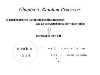
Chapter 5 Random Processes. ※ random process : a collection of time functions and an associated probability description marginal or joint pdf. How to extended the concepts of random variables

Chapter 5 Random Processes
E N D
Presentation Transcript
Chapter 5 Random Processes ※ random process : a collection of time functions and an associated probability description marginal or joint pdf
How to extended the concepts of random variables to those of random processes? simple • more difficult is to relate the mathematical representations for random variables to the physical properties of the process ※ classification of random processes continuous / discrete deterministic / nondeterministic stationary / nonstationary ergodic / nonergodic
5.2 Continuous & Discrete Random Processes • Dependent on the possible values of the random variables • continuous random process : ● random variables X(t1), X(t2), … can assume any value within a specified range of possible values ●PDF is continuous (pdf has NO δ function)
discrete random process : ● random variables can assume only certain isolated values ● pdf contains only δ functions • mixed process : have both continuous and discrete component
5.3 Deterministic & Non deterministic Random Processes random ftn of time • nondeterministic random process : future values of each sample ftn cannot be exactly predicted from the observed past values (almost all random processes are nondeterministic) • deterministic random process : ~ can be exactly predicted ~
(Example) X(t) = A cos(ωt + θ) A, ω … known constant θ … constant for all t but different for each sample function → random variation over the ensemble, not wrt time → still possible to define r.v. X(t1), X(t2), … and to determine pdf for r.v. Remark : convenient way to obtain a probability model for signals that are known except for one or two parameters
ensemble sample ftn X(t1) r.v. time t1 pdf 5.4 Stationary & Nonstationary Random Processes • dependency of pdf on the value of time • stationary random process: If all marginal and joint density function of the process do not depend on the choice of time origin, the process is said to be stationary (이 경우 모든 mean과 moment는 상수)
nonstationary random process: If any of the pdf does change with the choice of time origin, the process is nonstationary. All maginal & joint density ftn should be independent of the time origin! ⇒ too stringent ⇒ relaxed condition • mean value of any random variable X(t1) is independent of t1 & the correlation of two r.v. depends only on the time difference
random input response ⇒ stationary in the wide sense mean, mean-square, variance, correlation coefficient of any pair of r.v. are constant system analysis 결과는 strictly stationary 와 stationary in the wide sense의 두 경우 동일함! →구분하지 않고 사용
5.5 Ergodic & Nonergodic Random Process • If Almost every member of the ensemble shows the same statistical behavior as the whole ensemble, then it is possible to determine the statistical behavior by examining only one typical sample function. ⇒ Ergodic process
For ergodic process, the mean values and moments can be determined by time averages as well as by ensemble averages, that is, (Note) This condition cannot exist unless the process is stationary. → ergodic means stationary (not vice verse)
5.6 Measurement of Random Processes • Statistical parameters of a random process = the sets of statistical parameters associated with the r.v. X(t) at various times t these parameters are the same for all r.v. → consider only one set of parameters if stationary
How to estimate the process parameters from the observations of a single sample function? ← We cannot make an ensemble average for obtaining the parameters! if erogodic make a time average but, we cannot have a sample function over infinite time interval make a time average over a finite time interval approximation to the true value
※ Will determine • How good this approximation is? • Upon what aspects of measurement the goodness of the approximation depends? • Estimation of the mean value of an ergodic random process {X(t)} → random variable 이며 true mean value 와 같지 않음 → 얼마나 에 가까운가? 의 mean이 와 같고 variance가 작아야 함!
(see Ch.6) → T가 길수록 good estimate ! (Remark) 위의 계산을 위해선 X(t)의 표현식을 알아야 함 → 실제론 불가능 ⇒ discrete measurement를 취해서 해결
If we measure X(t) at equally spaced time interval , that is, then the estimate of can be expressed as mean mean-square
가정: statistically independent, that is, → mean of estimate = true mean
※ See the example in pp.201~202 zero-mean Gaussian Random process
5.7 Smoothing Data with a Moving Window Average A kind of LPF

