Navigable Small-World Networks

1. Navigable Small-World Networks Jim Dowling jdowling@kth.se Based on slides by ŠarūnasGirdzijauskas

2. Outline • Small-Worlds vs. Random Graphs • Navigation in Small-Worlds (Kleinberg’s model) • Small-World based Structured Overlays • Non-uniform Structured Overlays

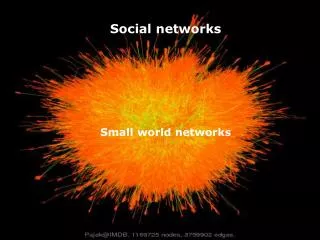
3. How is our society connected? • Structure of our social networks • Most people's friends are located in their vicinity, be it colleagues, neighbours, or team mates in the local soccer club. • Social networks were expected to be “grid-like“ • Within a specific social dimension (e.g., profession, hobby, geographical distribution) Implies the diameter of the social network is roughly O(√N).

4. Finding short chains of acquaintances linking pairs of people in USA who didn’t know each other; Source person in Nebraska and Kansas; Target person in Massachusetts. The letter could be only be given to persons one knows on a first name basis (acquaintances). Milgram’s(Small-World) experiment

5. Average length of the chains that were completed lied between 5 and 6 steps; Coined as “Six degrees of separation” principle. This was far less than assumed under the 'grid-like' assumption ! Similar results have been found in many other social networks BIG QUESTIONS: Why are there short chains of acquaintances linking together arbitrary pairs of strangers? That is, why is the diameter of the graph low? Milgram’s(Small-World) experiment

6. Random Graphs • Previously believed to be a Random graph • A random graph is a graph that is generated by some random process. • When pairs or vertices are joined uniformly at random -> then any two vertices are connected by a short chain with high probability. • However.. • If A and B have a common friend C it is likely that they themselves will be friends! (clustering) • Random networks tend not to be clustered

7. Graphs • A graph  G formally consists of a set of vertices V  and a set of edges E between them. That is, G=(V,E). • An edge connects vertex a with vertex b. • Edges can be directed or undirected. • The neighbourhoodN of a vertex a is defined as the set of its immediately connected vertices. • The degree of a vertex is defined as the number of vertexes in its neighbourhood. • Distance between two vertices is the number of edges in the shortest path connecting the vertices. • The diameter of a graph is maximum distance for any vertex.

8. Example Unidirected Graph b d a c

9. Regular Graph • A regular graph is a Graph where each vertex has the same number of neighbors • In other words, nodes have the same degree • Regular graphs can also be random • Random regular graph 2-regular graph 3-regular graph

10. Informally Clustering in Graphs • High clustering => a given vertex’s neighbours have lots of connections to each other • Low clustering => a given vertex’s neighbours have few connections to each other

11. Clustering coefficient • The local clustering coefficient C(v) of vertex v is a measure of how close v ‘s neighbours are to being a clique (a fully connected graph): where e(v) denotes the number of edges between the vertices in the v’sneighbourhood. • Network average clustering coefficient is given by the fraction of:

12. Clustering • Clustering measures the fraction of neighbours of a node that are connected among themselves • Regular Graphs have a high clustering coefficient • but also a high diameter • Random Graphs have a low clustering coefficient • but a low diameter • Both models do match some properties expected from real networks - such as Milgram’s!

13. Random vs. regular graphs • Long paths • L~N/(2k) • Highly clustered • C~3/4 • Short path length • L~logkN • Almost no clustering • C~k/N

14. Random rewiring procedure of regular graph (by Watts and Strogatz) With probability p rewire each link in a regular graph: Exhibit properties of both: random and regular graphs: High clustering coefficient; Low diameter. Small-World networks

15. This is still not enough to explain Milgram’sexperiment: If there exists a shortest path between any two nodes - where is the global knowledge that we can use to find this shortest path? Why should arbitrary pairs of strangers be able to find short chains of acquaintances that link them together? Why do decentralized “search algorithms” work? Small-World: remaining questions

16. Implications for P2P systems • Each P2P system can be interpreted as a directed graph where peers correspond to the nodes and their routing table entries as directed edges (links) to the other nodes

17. Implications for P2P systems • Task for P2P: • Invent a decentralized search algorithm that would route message from any node A to any other node B with relatively few hops compared with the size of the graph • Is it possible? • Milgram’s experiment suggests YES!

18. So why Milgram experiment worked? John, Stockholm; Neighbor; Musician; Likes photography; Etc. • A social network is not a simple graph, but a graph with certain “labels” • “labels“ representing various dimensions of our life • We internalize a “labeling space” with a distance metric! • We can greedily minimize the distance! • Decentralizedsearch: a greedy-routingalgorithm • We need to build the right graph where a decentralized search algorithm might perform the best Bill Simon, Paris; Friend; Stamp collector; Loves climbing; Etc. Peter, Stockholm; Colleague; Computer scientist; Loves movies; Etc.

19. Kleinberg’s model of Small-Worlds • Research of Jon Kleinberg: • Claim that there is no decentralized algorithm capable performing effective search in the class of SW networks according to Watts and Strogatz model; • J. Kleinberg presented the infinite family of Small World networks that generalizes Watts and Strogatz model and shows that decentralized search algorithms can find short paths with high probability; • It was proven that there exists only one unique model within that family for which decentralized search algorithms are effective.

20. Navigable Small-World networks • Kleinberg’s Small-World’s model • 2-dimensional lattice • Lattice (Manhattan) distance • Two type of edges: • Lattice edges (short range) • Long range • Probability for a node u to have a node v as a long range contact is proportional to

21. Influence of “r” • Each peer u has an edge to the peer v with probability where d(u,v) is the manhattan distance between u and v. • Tuning “r” • When r<dim (dimension of the euclidean space) we tend to choose more far away neighbours (search algorithm quickly approaches the target area, but slows down till it finally reaches the target). • When r>dim we tend to choose closer neighbours (search algorithm reaches the target area slowly if it is far away, but finds the target quickly in it’s neighbourhood). • When r=0 – long range contacts are chosen uniformly. Random graph theory proves there exists short paths between every pair of vertices, but there is no search algorithm capable of finding these paths. • When r=dim, the algorithm exhibits optimal performance.

22. Performance with r=dim • When q = 1 (there is one long range link) • The expected search cost is bounded by O(log2 N) • When q = k (there are a constant number of long range links) • The expected search cost is bounded by O(log2 N)/k • When q = log N • The expected search cost is bounded by O(log N)

23. How does it work in practice? • Normalization constant has to be calculated:

24. Example • Choose among 3 friends (1-dimension) • A (1 mile away) • B (2 miles away) • C (3 miles away) • Normalization constant

25. 0 1 1-dimensional continuous case • Peers uniformly distributed on a unit interval (or a ring structure) • Long range links chosen with the probability P~1/d • Search cost • O(log2N/k) with k long-range links • O(logN) with O(logN) long-range links • Systems: • Symphony (Manku et al, USITS 2003) • Accordion (Li et al, NSDI 2005)

26. 0.02 0.87 0.13 0.26 0.72 0.3 0.61 0.55 Small-World based P2P Overlay Systems: Symphony (Manku et al, USITS 2003) Accordion (Li et al, NSDI 2005) • Peersmapped onto positions on the ring • Uniform hash function (e.g., SHA-1) for peerId • Establish successor and predecessor ring links • Small-World connectivity establishment • No restrictions on peer-degree • Implicit load balancing

27. A1 A2 A3 A4 Approximation of Kleinberg’s model • Given node u if we can partition the remaining peers into sets A1, A2, A3, … , AlogN , where Ai, consists of all nodes whose distance from u is between 2-iand 2-i+1. • Then given r=dim each long range contact of u is nearly equally likely to belong to any of the sets Ai • When q=logN – on average each node will have a link in each set of Ai

28. Traditional DHTs and Kleinberg model • Most of the structured P2P systems are similar to Kleinberg’s model and are called logarithmic-like approaches. E.g. • Chord (randomized version) q=logN, r=1 • Gnutella q=5, r=0 • RandomizedChord’s model • Kleinberg’s model

29. Similarity to other P2P construction techniques • Many existing P2P are just the “special cases” of Kleinberg’s navigable Small-World • Ring based • Tree based • Hybercube • Torus • Etc., • Kleinberg’s Small-World • Randomized construction • No restrictions on peer-degree • “choice-of-two” possibility • Effective nonGreedy routing

30. What to take away from the small-world tour? • How can we characterize P2P overlay networks such that we can study them using graph-theoretic approaches? • What is the main difference between a random graph and a SW graph? • What is the main difference between Watts/Strogatz and Kleinberg models? • What is the relationship between structured overlay networks and small world graphs? • What are possible variations of the small world graph model? • How does it relate to our social networks?

31. Non-Uniform Structured Overlays

32. Structured overlay • Build a routing table • Each peer has a well-defined neighbourhood and information about its immediate neighbours (in contrast to unstructured topologies) • The search operation is performed efficiently (in contrast to unstructured)

33. 0.02 0.87 0.13 0.26 0.72 0.3 0.61 0.55 Data on a Ring-Structured Overlay • Peers mapped onto an ID the ring identifier space • Uniform hash function (e.g., SHA-1) • Resources mapped on to an ID the ring identifier space • Uniform hash function • Peers are responsible for a range of the ring identifier space • Connectivity establishment • E.g., Symphony [Manku et al. 2003] • Uniform peer key (id) distribution • Implicit load balancing

34. Problems with range queries • Point queries • E.g. “ABBA Waterloo” • “ABBA Mamma Mia” • Range queries: • What about all the files with prefix “ABBA..”? • Uniform hashing assigns all the files to random locations on the ring • Uniform distribution of IDs (keys) • Inefficient lookup! • Order preserving (Lexicographic) hashing • If a > b then id(a)>id(b) (in uniform hashing id(a)=rand; id(b)=rand) • Non-uniform distribution (depends on the data)!

35. Problems with uniform key distributions • Order preserving hash functions (e.g. Lexicographical ordering) • Peer clustering in key space Etc. • For skewed key distributions • How do we make SW long range links?

36. Extending Kleinberg’s model Stretched spaceOriginal space

37. Extension of the “uniform model” to nonuniform case (1)

38. Small-World P2P in non-uniform spaces • f(x) – probability density function of the peer keys. • Long range neighbours are chosen inversely proportional to the integral of f(x) between the two nodes Expected routing cost in such a network using greedy routing is O(log N) when the network degree is O(log N).

39. Acquiring Peer Key Distribution • Problem: • Need to acquire the global key distribution function locally. • Uniform sampling • (Mercury[Bharambe et al.,2004]) • log2N samples • Cannot cope with • complex distributions!  • Non-uniform (Scalable Sampling) • OSCAR (Overlays using SCAlable sampling of Realistic distributions) • [DBISP2P06, ICDE07, TAAS10]

40. Sampling by random walks • Bharambe et al. 2004 ”Mercury: supporting scalable multi-attribute range queries” • Sampling by random walks • A random walk with TTL at least logN ends up in a uniform random node (on expander graphs)

41. Sampling in Mercury • Every node periodically issues k1 samples • The sampled nodes return its ID and their own collected samples (k2) • It is suggested k1=logN • Over time the ID distribution histogram is built. • Real world distributions are far more complex!

42. Oscar: Modifying Kleinberg’s method • Choosing long-range link: 1) u.a.r. choose a partition 2) u.a.r. choose a peer within that partition • It can be proven that search cost remains O(log2N) O(logN) with O(logN) degree

43. Oscar: Dealing with Skewed Spaces • Find the boundaries between partitions! • Uniform sampling by random walks. • k samples for each boundary.

44. Oscar: an Example 0 1 • O(k*log N) samples is needed to construct a routing efficient network. • Does not depend on the complexity of the distribution • “The view” can be copied from a ring-neighbour • (by contacting median peers and requesting their ring-neighbourids)

45. Recap of non-uniform structured overlays • What is the relationship between the resource placement and the network structure in structured P2P overlays? • What is a challenge for enabling range queries for structured overlays? • What is the main difference between a regular Kleinberg’s model Small-World model for non-uniform id spaces? • How does random sampling work? • What are the possible solutions to solve the non-uniform resource placement problem? Acknowledgements: Someslideswerederivedfrom the lecture notes of K. Aberer (EPFL, Switzerland) and A. Datta (NTU, Singapore)