Modeling Heterogeneity in Production Functions: Stochastic Frontier and Inefficiency Analysis
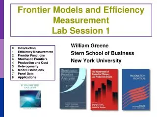
This session at the William Greene Efficiency Measurement Course focuses on modeling heterogeneity within production function models incorporating inefficiency through stochastic frontier models. Key topics include the Normal-Half-Normal model, skewness in OLS residuals, cost inefficiency, and duality in production vs. cost frontiers. The session emphasizes Bayesian treatments, empirical applications using panel data, and addresses observable vs. unobservable heterogeneity in production processes. Insights from various studies and examples, including the healthcare sector, will provide practical understanding of inefficiency dynamics.

Modeling Heterogeneity in Production Functions: Stochastic Frontier and Inefficiency Analysis
E N D
Presentation Transcript
William Greene Stern School of Business New York University Efficiency Measurement
Session 5 Modeling Heterogeneity
The Stochastic Frontier Model ui > 0, but vi may take any value. A symmetric distribution, such as the normal distribution, is usually assumed for vi. Thus, the stochastic frontier is +’xi+vi and, as before,ui represents the inefficiency.
Log Likelihood Function Waldman (1982) result on skewness of OLS residuals: If the OLS residuals are positively skewed, rather than negative, then OLS maximizes the log likelihood, and there is no evidence of inefficiency in the data.
Fundamental Tool - JLMS We can insert our maximum likelihood estimates of all parameters. Note: This estimates E[u|vi – ui], not ui.
Cost Inefficiency y* = f(x) C* = g(y*,w) (Samuelson – Shephard duality results) Cost inefficiency: If y < f(x), then C mustbe greater than g(y,w). Implies the idea of a cost frontier. lnC = lng(y,w) + u, u > 0.
Where to Next? • Heterogeneity: “Where do we put the z’s?” • Other variables that affect production and inefficiency • Enter production frontier, inefficiency distribution, elsewhere? • Heteroscedasticity • Another form of heterogeneity • Production “risk” • Bayesian and simulation estimators • The stochastic frontier model with gamma inefficiency • Bayesian treatments of the stochastic frontier model • Panel Data • Heterogeneity vs. Inefficiency – can we distinguish • Model forms: Is inefficiency persistent through time? • Applications
Observable Heterogeneity • As opposed to unobservable heterogeneity • Observe: Y or C (outcome) and X or w (inputs or input prices) • Firm characteristics z. Not production or cost, characterize the production process. • Enter the production or cost function? • Enter the inefficiency distribution? How?
Shifting the Outcome Function Firm specific heterogeneity can also be incorporated into the inefficiency model as follows: This modifies the mean of the truncated normal distribution yi = xi + vi - ui vi ~ N[0,v2] ui = |Ui| where Ui ~ N[i, u2], i = 0 + 1zi,
One Step or Two Step 2 Step: Fit Half or truncated normal model, compute JLMS ui, regress ui on zi Airline EXAMPLE: Fit model without POINTS, LOADFACTOR, STAGE 1 Step: Include zi in the model, compute ui including zi Airline example: Include 3 variables Methodological issue: Left out variables in two step approach.
One vs. Two Step 0.8 0.9 1.0 Efficiency computed without load factor, stage length and points served. Efficiency computed with load factor, stage length and points served.
Unobservable Heterogeneity • Parameters vary across firms • Random variation (heterogeneity, not Bayesian) • Variation partially explained by observable indicators • Continuous variation – random parameter models: Considered with panel data models • Latent class – discrete parameter variation
Latent Class Efficiency Studies • Battese and Coelli – growing in weather “regimes” for Indonesian rice farmers • Kumbhakar and Orea – cost structures for U.S. Banks • Greene (Health Economics, 2005) – revisits WHO Year 2000 World Health Report • Kumbhakar, Parmeter, Tsionas (JE, 2013) – U.S. Banks.
Inefficiency? • Not all agree with the presence (or identifiability) of “inefficiency” in market outcomes data. • Variation around the common production structure may all be nonsystematic and not controlled by management • Implication, no inefficiency: u = 0.
Nursing Home Costs • 44 Swiss nursing homes, 13 years • Cost, Pk, Pl, output, two environmental variables • Estimate cost function • Estimate inefficiency
A Two Class Model • Class 1: With Inefficiency • logC = f(output, input prices, environment) + vv + uu • Class 2: Without Inefficiency • logC = f(output, input prices, environment) + vv • u = 0 • Implement with a single zero restriction in a constrained (same cost function) two class model • Parameterization: λ = u /v = 0 in class 2.
LogL= 464 with a common frontier model, 527 with two classes
Heteroscedasticity in v and/or u Var[vi | hi] = v2gv(hi,) = vi2 gv(hi,0) = 1, gv(hi,) = [exp(’hi)]2 Var[Ui | hi] = u2gu(hi,)= ui2 gu(hi,0) = 1, gu(hi,) = [exp(’hi)]2
Unobserved Endogenous Heterogeneity • Cost = C(p,y,Q), Q = quality • Quality is unobserved • Quality is endogenous – correlated with unobservables that influence cost • Econometric Response: There exists a proxy that is also endogenous • Omit the variable? • Include the proxy? • Question: Bias in estimated inefficiency (not interested in coefficients)
Simulation Experiment • Mutter, et al. (AHRQ), 2011 • Analysis of California nursing home data • Estimate model with a simulated data set • Compare biases in sample average inefficiency compared to the exogenous case • Endogeneity is quantified in terms of correlation of Q(i) with u(i)
A Simulation Experiment Conclusion: Omitted variable problem does not make the bias worse.


